Higher-order character decomposition: char module#
NOTE: This tutorial assumes familiarity with the concepts explained in Conceptual and mathematical background of higher-order Fourier analysis and that the
HoFapackage has already been installed, see Installation.
In this notebook we are going to learn how the HoFa package identifies higher-order components of a function.
What are higher-order characters?#
As we saw in Conceptual and mathematical background of higher-order Fourier analysis, the question of what are the higher-order components of a function is a subtle one, especially because, once we go beyond classical Fourier analysis, we lose the concept of exactness and replace it with the concepts of sparsity and efficiency.
This was illustrated in the quadratic setting where we saw that, when working with the Gowers \(U^3\)-norm, the family of classical Fourier characters such as
needs to be enlarged to include, among what we expect to call quadratic characters, functions such as quadratic waves of the form
This already shows that quadratic characters are too numerous to form a basis of our vector space of functions. This is one sense in which we have the above-mentioned loss of exactness (we lose the concept of a basis, and its associated ability to give exact decompositions of functions as linear combinations of basis elements).
Moreover, it is known (as we discuss in Theoretical foundations and extensions) that quadratic characters must also include functions that can be more subtle than these quadratic waves, such as 2-step nilsequences.
Nevertheless, there is a relatively simple and natural notion of quadratic character (or, more generally, of \((k-1)\)-th order character, if we work with the \(U^{k+1}\)-norm), which happens to capture all these examples. We discussed these quadratic characters in the U3-norm case in the Conceptual background, and saw that they are defined by the property that their multiplicative derivatives should be structured functions in the classical Fourier sense, namely, they should be well-approximated by linear combinations of a few classical Fourier characters. This notion generalizes also naturally to higher orders, leading to the idea of a character of order \(k\) being a function whose multiplicative derivatives are structured functions of order \(k-1\).
The general goal: find the dominant higher-order characters of a function#
Recent theoretical results indicate that functions on finite abelian groups can be decomposed, up to error terms that are small in either the Euclidean norm or the Gowers \(U^{k+1}\)-norm, by sums of a few order-\(k\) characters (see Theoretical foundations and extensions).
The purpose of this tutorial is to explore how the HoFa package can compute such decompositions of a function \(f\), namely decompositions of the form \(f=f_e+\sum g_i\) where \(f_e\) is an error term and the \(g_i\) are characters of order \(k\). We shall focus on the quadratic case.
Similarly as for the hofa.rgz.regularize method, these decompositions depend on tunable parameters. While the package includes default heuristics for selecting these parameters, practitioners are encouraged to experiment with different strategies for their specific applications.
REMARK. Recall that the Discrete Fourier Transform gives a unique decomposition for functions on (say) \(\mathbb{Z}/n\mathbb{Z}\). In particular, any higher-order Fourier character can be decomposed uniquely as some linear combination of Fourier characters. However, in general, this decomposition is not sparse or efficient. Thus, decompositions into a few higher-order characters can often be much sparser than classical Fourier decompositions.
A simple example: identifying a single quadratic character#
Let us begin by importing the necessary libraries. Recall that we are assuming that the HoFa package is already installed, see Installation. For a quick installation, run the following command:
(hofavenv) $ pip install hofa
import numpy as np
import matplotlib.pyplot as plt
np.set_printoptions(precision=5)

import hofa.char as char
import hofa.rgz as rgz
import hofa.cdf as cdf
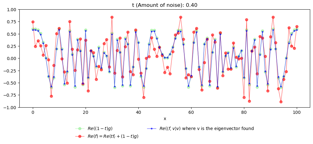
Consider a single quadratic character \(g(x):=e^{2\pi i x^2/n}\), for \(x=0,\ldots,n-1\). As usual, suppose that we perturb it with some random noise \(f_r(x)\sim \text{Unif}[-1,1)\) in a way that we can only see the convex combination \(f:=tf_r+(1-t)g\) for \(t=0.4\).
n = 101
t = 0.4

rng = np.random.default_rng(seed=123)

x = np.arange(n)
g = np.exp(2*1j*np.pi*x**2/n)

f = rng.uniform(-1, 1, size=len(x))*t+(1-t)*g
The hofa.char module contains a method spechoft (Spectral higher-order Fourier transform) which enables us to recover the underlying structured component \((1-t)g\). It returns data related to finding those characters, but the most important part is the attribute higher_order_char, which is a numpy.ndarray of shape (f.shape,m) where m represents the number of components (higher-order characters) found.
If we represent the higher_order_char result of spechoft as a family of vectors \(v_i\), the resulting higher-order character decomposition of \(f\) is as follows:
NOTE: Recall that the default use of
spechoftutilizes some heuristics for some tunable parameters. We will learn below how to modify these parameters and obtain different decompositions for the same function.
In our case, since we know that the function \(f\) in our example will contain exactly one higher-order character, we simply define v below as such an element.
v = char.spechoft(f, rng=123).higher_order_char[...,0]

coeff_proj = np.mean(f*v.conjugate())

error = np.mean(np.abs(g*(1-t)-coeff_proj*v))
print(r'L1 error between the known quadratic Fourier character (1-t)g and <f,v>v : '+str(error))
L1 error between the known quadratic Fourier character (1-t)g and <f,v>v : 0.02255730958724428
As we can see, the error is very small and, up to the scaling factor \((1-t)\), we are able to recover the character \(g\).
Let us plot below the (real part of the) original function \((1-t)g\), the (real part of the) noisy version \(f\), and the (real part of the) reconstruction which comes from the projection of \(f\) to the (sole) eigenvector returned by spechoft.
fig, ax = plt.subplots(figsize=(12, 5))

# Plot original (1-t)*f_s in light green
ax.plot(x, np.real(g*(1-t)), linestyle='-', color='lightgreen', marker='o', markersize=6, linewidth=1, alpha=0.6, label=r'$Re((1-t)g)$')

# Plot modified function in red
ax.plot(x, np.real(f), linestyle='-', color='red', marker='o', markersize=6, linewidth=1, alpha=0.6, label=r'$Re(f) = Re(tf_r+(1-t)g)$')

# Plot recovered function in blue
ax.plot(x, np.real(coeff_proj*v), linestyle='-', color='blue', marker='o', markersize=3, linewidth=1, alpha=0.6, label=r'$Re(\langle f,v\rangle v)$ where v is the eigenvector found')

# Customize the plot
ax.set_xlabel("x")
ax.set_title(f"t (Amount of noise): {t:.2f}")
ax.set_ylim(-1,1)

# Legend below the plot
fig.subplots_adjust(bottom=0.25)  # Adjust layout to fit legend below
ax.legend(loc='upper center', bbox_to_anchor=(0.5, -0.15), ncol=2, frameon=False)

# Show the plot
plt.show()
This first example may not seem very impressive since, after all, we already know a method from the hofa package that can recover the original character, namely hofa.rgz.regularize (indeed this method recovers this single character simply as the regularized version of the function \(f\)).
The real challenge begins when there are several higher-order characters that cannot be distinguished by simply applying hofa.rgz.regularize. The next example illustrates a method from hofa.char which achieves this distinction.
A first multi-character example#
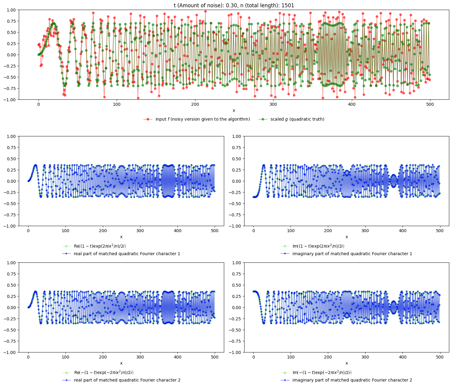
Let \(g(x):=\sin(2\pi x^2/n)\) and, as above, let \(f_r(x)\sim \text{Unif}[-1,1)\). Again, assume that we are presented with a noisy version \(f:=tf_r+(1-t)g\) for some \(t\in[0,1)\).
Returning to our intuition with quadratic Fourier characters, it is reasonable to aim to decompose \(g\) as follows:
Equivalently, the quadratic characters hidden in \(f\) that we want to extract are \((1-t)\exp(2\pi i x^2/n)/2i\) and \(-(1-t)\exp(-2\pi i x^2/n)/2i\).
n = 1501
t = 0.3

x = np.arange(n)
g = np.sin(2*np.pi*x**2/n)

# We fix a seed for reproducibility
rng = np.random.default_rng(seed=28)
f = rng.uniform(-1, 1, size=len(x))*t+(1-t)*g
The method char.spechoft is specifically designed to identify and extract such components.
# As usual, we fix an rng for reproducibility
rnd_sep_result = char.spechoft(f, rng=28)

eichars = rnd_sep_result.higher_order_char
The attribute higher_order_char contains an array of the quadratic Fourier characters that compose the structured part of \(f\), i.e., \((1-t)g\). In this example (try it in your notebook!), you will find exactly two characters, which correspond to the two quadratic Fourier characters that make up \(g\).
Below, we visualize the key elements of this example. For clarity, we first plot the real-valued functions \(f\) and \((1-t)g\). For the quadratic Fourier characters and the extracted quadratic components, we plot both their real and imaginary parts.
Note that, similarly to what happens with the standard Fourier transform (which uses complex exponentials as Fourier characters), here even if the function to decompose is real-valued (e.g., \(f\) or \((1-t)g\)), its decomposition may still involve complex numbers.
import itertools
import numpy as np
import matplotlib.pyplot as plt

number_of_first_elems_to_plot = 500

v_1 = eichars[:, -1]
coeff_proj_1 = np.mean(f * v_1.conjugate())

v_2 = eichars[:, -2]
coeff_proj_2 = np.mean(f * v_2.conjugate())

# Restrict to plotting window
x_plot = x[:number_of_first_elems_to_plot]

# Target ("green") complex curves
target_1_complex = (1 - t) * np.exp(2 * np.pi * 1j * x_plot**2 / n) / (2*1j)
target_2_complex = -(1 - t) * np.exp(-2 * np.pi * 1j * x_plot**2 / n) / (2*1j)

targets_complex = [target_1_complex, target_2_complex]

# Recovered ("blue") complex curves
blue_1_complex = coeff_proj_1 * v_1[:number_of_first_elems_to_plot]
blue_2_complex = coeff_proj_2 * v_2[:number_of_first_elems_to_plot]

blues_complex = [blue_1_complex, blue_2_complex]

# --- L^2 (squared) error comparison over all possible assignments ---

best_perm = None
best_err = np.inf

for perm in itertools.permutations(range(2)):
    total_err = sum(
        np.sum(np.abs(blues_complex[perm[i]] - targets_complex[i])**2)
        for i in range(2)
    )
    if total_err < best_err:
        best_err = total_err
        best_perm = perm

# Reorder blues according to best assignment
matched_blues_complex = [blues_complex[best_perm[i]] for i in range(2)]

# Labels
target_labels_real = [
    r'$\mathrm{Re}\!\left((1-t)\exp(2\pi i x^2/n)/2i\right)$',
    r'$\mathrm{Re}\!\left(-(1-t)\exp(-2\pi ix^2/n)/2i\right)$',
]

target_labels_imag = [
    r'$\mathrm{Im}\!\left((1-t)\exp(2\pi i x^2/n)/2i\right)$',
    r'$\mathrm{Im}\!\left(-(1-t)\exp(-2\pi ix^2/n)/2i\right)$',
]

blue_labels_real = [
    r"real part of matched quadratic Fourier character 1",
    r"real part of matched quadratic Fourier character 2",
]

blue_labels_imag = [
    r"imaginary part of matched quadratic Fourier character 1",
    r"imaginary part of matched quadratic Fourier character 2",
]

# --- Plotting ---

# 4 rows x 2 columns:
# top row spans both columns,
# then 3 rows of 2 plots each
fig = plt.figure(figsize=(15, 16))
gs = fig.add_gridspec(4, 2, height_ratios=[1, 1, 1, 1], width_ratios=[1, 1])

# Top plot
ax_top = fig.add_subplot(gs[0, :])
ax_top.plot(
    x_plot,
    f[:number_of_first_elems_to_plot],
    linestyle="-",
    color="red",
    marker="o",
    markersize=5,
    linewidth=1,
    alpha=0.6,
    label=r"input $f$ (noisy version given to the algorithm)",
)
ax_top.plot(
    x_plot,
    (1 - t) * g[:number_of_first_elems_to_plot],
    linestyle="-",
    color="green",
    marker="o",
    markersize=5,
    linewidth=1,
    alpha=0.6,
    label=r"scaled $g$ (quadratic truth)",
)
ax_top.set_xlabel("x")
ax_top.set_title(f"t (Amount of noise): {t:.2f}, n (total length): {n}")
ax_top.set_ylim(-1, 1)
ax_top.legend(loc="upper center", bbox_to_anchor=(0.5, -0.15), ncol=2, frameon=False)

# Bottom 3x2 comparison plots
for i in range(2):
    target = targets_complex[i]
    blue = matched_blues_complex[i]

    # Left: real parts
    ax_real = fig.add_subplot(gs[i + 1, 0])
    ax_real.plot(
        x_plot,
        np.real(target),
        linestyle="-",
        color="lightgreen",
        marker="o",
        markersize=5,
        linewidth=1,
        alpha=0.6,
        label=target_labels_real[i],
    )
    ax_real.plot(
        x_plot,
        np.real(blue),
        linestyle="-",
        color="blue",
        marker="o",
        markersize=3,
        linewidth=1,
        alpha=0.6,
        label=blue_labels_real[i],
    )
    ax_real.set_xlabel("x")
    ax_real.set_ylim(-1, 1)
    ax_real.legend(loc="upper center", bbox_to_anchor=(0.5, -0.15), ncol=1, frameon=False)

    # Right: imaginary parts
    ax_imag = fig.add_subplot(gs[i + 1, 1])
    ax_imag.plot(
        x_plot,
        np.imag(target),
        linestyle="-",
        color="lightgreen",
        marker="o",
        markersize=5,
        linewidth=1,
        alpha=0.6,
        label=target_labels_imag[i],
    )
    ax_imag.plot(
        x_plot,
        np.imag(blue),
        linestyle="-",
        color="blue",
        marker="o",
        markersize=3,
        linewidth=1,
        alpha=0.6,
        label=blue_labels_imag[i],
    )
    ax_imag.set_xlabel("x")
    ax_imag.set_ylim(-1, 1)
    ax_imag.legend(loc="upper center", bbox_to_anchor=(0.5, -0.15), ncol=1, frameon=False)

fig.tight_layout()
plt.show()
How the algorithm works#
Recall from Tutorial - Denoising (regularization), rgz and cdf that the regularization process implemented in hofa.rgz.regularize involves, for a given function \(f\), finding significant (i.e. large) eigenvalues of a matrix \(\mathcal{K}(f \otimes \overline{f})\) and then projecting \(f\) to the linear span of the corresponding eigenvectors.
It is natural to expect that these eigenvectors themselves are the desired higher-order characters underlying \(f\). However, as we will see in the following example, this is not always the case. This example is phrased in the context of classical Fourier analysis. Nevertheless, the quadratic case follows a similar intuition, making this example enlightening for understanding both scenarios.
Why separation of eigenvalues is needed#
Let \(n\) be a positive integer, and let \(f:\{0,\ldots,n-1\}\to \mathbb{C}\) be the function defined by \(f(x) = \cos(2\pi x/n)\). Suppose we want to find the Fourier components of this function using only the regularization algorithm and linear algebra, without prior knowledge of the Fourier characters on the interval \(\{0,\ldots,n-1\}\).
When using hofa.rgz.regularize with order=1, the algorithm constructs the matrix \(\mathcal{K}(f \otimes \overline{f})\), which is equal to:
where \(\chi_1(x) = \exp(2\pi i x/n)\) and \(\chi_2(x) = \exp(-2\pi i x/n)\).
Note: The interested reader may try to derive this result. The idea is to apply the averaging operator to each diagonal, replacing each \(Z\)-diagonal with its average value.
From a linear algebra perspective, the matrix \(\mathcal{K}(f \otimes \overline{f})\) is a rank-2 matrix with two eigenvectors, both sharing the same eigenvalue \(\tfrac{1}{4}\). Thus, its spectral decomposition reveals:
A single eigenspace of dimension 2 associated with the eigenvalue \(\tfrac{1}{4}\).
Another eigenspace of dimension \(n-2\) associated with the eigenvalue \(0\).
This poses a problem for identifying the individual Fourier characters \(\chi_1\) and \(\chi_2\). Indeed we only observe a single eigenspace, and in practical terms, if we use a linear algebra module to compute the eigenvalues and eigenvectors of this matrix, we obtain the correct eigenvalues, but the eigenvectors are just some linear combinations of the desired characters, and typically not the characters themselves.
A solution: random sampling and iteration#
Starting from the previous example, once we have identified the eigenspace generated by \(\chi_1\) and \(\chi_2\), we can randomly sample a vector of modulus 1 from this eigenspace. Such a vector will have the form:
The critical observation is that, with probability 1, we have \(|c| \neq |d|\). If we then apply the method hofa.rgz.regularize (with order=1) to the function \(c \chi_1 + d \chi_2\), the corresponding matrix becomes:
Now, we have two distinct eigenspaces with different eigenvalues. As a result, any linear algebra method will correctly identify \(\chi_1\) and \(\chi_2\) as the eigenvectors.
How the separation process works in higher orders#
As we have seen before, exact results in classical Fourier analysis translate to approximate results in higher-order Fourier analysis. Thus, concepts such as having different eigenvalues become having eigenvalues sufficiently separated, and with probability 1 becomes with high probability. In this spirit, let us present a minimalistic pseudocode describing how the function hofa.char.spechoft works.
Minimalistic pseudocode of the spectral higher-order Fourier transform
Input: Function to process: \(f: Z \to \mathbb{C}\) and order of regularization \(k\).
Initial regularization:
\(f_{\text{reg,init}},\{(\lambda,v): \text{ pairs of eigenvalues/eigenvectors}\} \leftarrow \text{regularize}(f,k)\)
\(\rho_{\text{init}} \leftarrow \text{initial\_threshold}(f, f_{\text{reg,init}})\)
\(N_{\text{target}} \leftarrow \# \{\lambda \text{ greater than } \rho_{\text{init}} \}\)
Initialization for the loop:
\(h \leftarrow f_{\text{reg,init}}\quad\)
\(\text{are\_separated} \leftarrow \text{False}\)
While \(\text{are\_separated} == \text{False} \):
\(f_{\text{reg,iter}}, \{(\lambda',v'): \text{ pairs of eigenvalues/eigenvectors}\} \leftarrow \text{regularize}(h,k)\)
\(\rho_{\text{iter}} \leftarrow \text{iteration\_threshold}(h, f_{\text{reg,iter}})\)
\(N_{\text{found}} \leftarrow \# \{\lambda' \text{ greater than } \rho_{\text{iter}} \}\)
If \(N_{\text{found}} == N_{\text{target}}\):
\(\text{are\_separated} \leftarrow \text{are\_eigenvalues\_sufficiently\_separated}(\{\lambda': \lambda' \ge \rho_{\text{iter}}\})\)
If \(\text{are\_separated} == \text{False}\):
\(h \leftarrow \text{random\_unit\_vector}(\{v: \text{ corresponding }\lambda\ge \rho_{\text{init}} \})\)
Output: \(\{v': v'\ge \rho_{\text{iter}}\}\) found in Step 3.A.
The decomposition of \(f\) into the different higher-order Fourier characters will be of the following form:
where the term \(\langle f, v'\rangle v'\) are the higher-order Fourier characters in the decomposition of \(f\) and \(f_e\) is the error term.
Refinements of the algorithm#
While the pseudocode captures the core logic of hofa.char.spechoft, the actual implementation includes several practical refinements to ensure robustness, efficiency, and flexibility. Below, we describe how each step of the pseudocode is adapted in the implementation:
Refining Step 1 (the initial regularization)#
Step 1.A: Similar to
hofa.rgz.regularize,hofa.char.spechoftenables the user to pass a list ofhofa.rgz.LayerRegularizerobjects to perform the initial regularization of \(f\). This provides flexibility in choosing the regularization method.Step 1.B: A threshold must be computed to determine eigenvalue separation.
hofa.char.spechoftis designed so that the user can define how this threshold is calculated.
Refining Step 3: iterative refinement#
Termination Condition: The loop in the pseudocode could run indefinitely. To prevent this,
hofa.char.spechoftrequires the user to specify a maximum number of iterations, which may depend on \(f\) and the initial regularization \(f_{\text{reg,init}}\).Step 3.A: A second regularization is performed on \(h\) (initially \(f_{\text{reg,init}}\) and updated in subsequent iterations). The user can specify a different regularization procedure for this step, distinct from the one used in Step 1.A.
Step 3.B: As in Step 1.B, a threshold must be computed to determine when eigenvectors are sufficiently separated.
hofa.char.spechoftenables the user to define how this threshold is calculated.Step 3.D: Eigenvalue Separation Strategy
hofa.char.spechoftsupports two approaches for handling eigenvalue separation:Strict Separation: Declare success only if all eigenvalues of \(h\) are sufficiently separated.
Iterative Search: For a given \(h\), if the eigenvectors \(v_1, \ldots, v_m\) have sufficiently large and separated eigenvalues, record these eigenvectors and update \(f\) as: $\( f \leftarrow f - \sum_{i=1}^m \langle f, v_i \rangle v_i. \)$ This approach progressively isolates fewer components in each iteration.
This design ensures that hofa.char.spechoft is both flexible (allowing user-defined thresholds and regularization methods) and robust (avoiding infinite loops and efficiently isolating components).
The role of randomization#
Randomization plays a crucial role in the algorithm, as for the general higher-order case we cannot rely on a priori knowledge of the structure of higher-order characters (in contrast to what happens for the case of classical Fourier analysis). Fortunately, eigenvalues act as detectors of when certain eigenvectors represent real higher-order Fourier characters. The details of why this holds in the general case are analogous to the case of classical Fourier analysis, but the theoretical justification is much more complicated. The interested reader is invited to check the original paper and/or contact the authors of this package for further details.
Convergence and termination#
The algorithm terminates when one of the following conditions is met:
Success: All target higher-order characters have been successfully separated, either iteratively or all at once.
Iteration Limit: The maximum number of iterations is reached without success.
The iterative approach, where successfully separated components are recorded and removed from further consideration, significantly improves the algorithm’s efficiency.
The random separator policy#
The algorithm’s flexibility is implemented via a policy object that encapsulates the strategy for determining Algorithmic refinements. This is where the hofa.char.RandomSeparator abstract base class comes into play. Its purpose is to determine:
Initial Threshold: How to compute the starting minimum threshold for identifying potential higher-order components.
Iteration Threshold: How to compute the minimum thresholds during the iterative refinement process.
Separation Gap: How to determine when eigenvalues are sufficiently separated.
Iteration Control: How many iterations to perform.
Iterative search: whether to remove already found characters or to try to find a candidate random function such that all its significant eigenvalues are already sufficiently separated.
This encapsulation of the policy object allows the core algorithm in hofa.char.spechoft to remain generic while enabling customization through different separator implementations.
The class hofa.char.RandomSeparator#
Let us see the definition in Python of this abstract class.
# In hofa.char
class RandomSeparator(ABC):
    @abstractmethod
    def initial_threshold(self, f: np.ndarray, reg_res: rgz.RegularizationResult) -> float:
        """Compute the initial threshold for eigenvalue separation."""

    @abstractmethod
    def iteration_threshold(self, f: np.ndarray, reg_res: rgz.RegularizationResult,
                        initial_f: np.ndarray, initial_reg_res: rgz.RegularizationResult) -> float:
        """Compute the threshold for each iteration of the separation process."""

    @abstractmethod
    def separation_gap(self, f: np.ndarray, reg_res: rgz.RegularizationResult,
                   initial_f: np.ndarray, initial_reg_res: rgz.RegularizationResult) -> float:
        """Compute the gap required between eigenvalues for successful separation."""

    @abstractmethod
    def get_rng(self) -> np.random.Generator:
        """Get the random number generator used by this object."""

    @abstractmethod
    def max_iter(self, f: np.ndarray, reg_res: rgz.RegularizationResult) -> int:
        """Get the maximum number of iterations for the separation process."""

    @abstractmethod
    def iterative_search(self) -> bool:
        """Determine whether the algorithm should use iterative search."""
Let us examine now each method of the RandomSeparator interface in detail, explaining their roles in the spectral decomposition algorithm and how they interact with each other during execution.
Initial threshold calculation#
@abstractmethod
def initial_threshold(self, f: np.ndarray, reg_res: rgz.RegularizationResult) -> float:
Purpose:
This method computes the initial threshold used to identify potential higher-order characters in the first phase of the algorithm. The threshold determines which eigenvalues of the regularized function are considered significant enough to potentially represent higher-order characters. In the pseudocode of the minimalistic spectral higher-order Fourier transform, the returned value corresponds to \(\rho_{\text{init}}\) in Step 1.B.
Parameters:
f: The original input function before regularization.reg_res: The result of regularizingf, including the different eigenvalues and eigenvectors.
Returns:
A float value representing the computed threshold.
Implementation notes:
Subclasses should implement this method to return a threshold that balances between:
Including all potential higher-order characters (threshold too low).
Excluding noise and insignificant components (threshold too high).
Iteration threshold calculation#
@abstractmethod
def iteration_threshold(self, f: np.ndarray, reg_res: rgz.RegularizationResult,
                      initial_f: np.ndarray, initial_reg_res: rgz.RegularizationResult) -> float:
Purpose:
This method computes the threshold used during each iteration of the separation process. Unlike the initial threshold, this threshold may adapt to the current state of the algorithm. In the pseudocode of the minimalistic spectral higher-order Fourier transform, the returned value corresponds to \(\rho_{\text{iter}}\) in Step 3.B.
Parameters:
f: The current function being analyzed.reg_res: The regularization result off.initial_f: The original input function (for reference).initial_reg_res: The initial regularization result (for reference).
Returns:
A float value representing the computed iteration-specific threshold.
Separation gap calculation#
@abstractmethod
def separation_gap(self, f: np.ndarray, reg_res: rgz.RegularizationResult,
                 initial_f: np.ndarray, initial_reg_res: rgz.RegularizationResult) -> float:
Purpose:
This method determines when an eigenvalue is sufficiently separated from the rest of significant eigenvalues. If we denote by \(\Delta\) the output of this method, the function hofa.char.spechoft will consider \(\lambda\) separated if it has multiplicity 1 and there are no other eigenvalues in the interval \((\lambda-\Delta,\lambda+\Delta)\). That is, in the pseudocode of the Minimalistic spectral higher-order Fourier transform, the returned value \(\Delta\) will be used in Step 3.D to determine whether some or all (depending on whether we use the iterative approach or not) large eigenvalues (i.e. larger than \(\rho_{\text{iter}}\)) are separated from the rest (i.e. they have multiplicity 1 and there is no other eigenvalue in the interval \((\lambda-\Delta,\lambda+\Delta)\)).
Parameters:
Same as iteration_threshold.
Returns:
A float value representing the minimum required gap between large eigenvalues.
Implementation notes:
Choosing an appropriate method for computing the separation gap is important because:
A value too large will make it impossible for eigenvalues to be declared separated, so that the algorithm will most likely finish without success.
A value too small will run into problems of not finding genuine higher-order Fourier characters, as some separation of the eigenvalues is needed.
Random number generator access#
def get_rng(self) -> np.random.Generator:
Purpose:
This method provides access to the random number generator used internally by the separator. This allows for reproducible results and gives users control over the randomization process.
Returns:
The numpy.random.Generator instance used by this object.
Implementation notes:
The random number generator (RNG) should be properly initialized during object construction.
Users can inspect or modify the RNG state if needed (though modifying it may affect reproducibility)
Maximum iterations#
def max_iter(self, f: np.ndarray, reg_res: rgz.RegularizationResult) -> int:
Purpose:
This method determines the maximum number of iterations allowed for the separation process. It provides a way to control the trade-off between computation time and result quality.
Parameters:
f: Current function.reg_res: Current regularization result.
Returns:
The maximum number of iterations to perform.
Implementation notes:
The default implementation typically returns a fixed value set during initialization. Subclasses can override this to implement dynamic determination based on:
The size or complexity of the input data.
Computational constraints.
This method ensures the algorithm terminates even if separation is not achieved.
Iterative search flag#
def iterative_search(self) -> bool:
Purpose:
This method indicates whether the algorithm should use an iterative approach to find higher-order characters. The iterative approach is generally more efficient than trying to find all components at once.
Returns:
True if iterative search should be used, False otherwise.
Implementation notes:
Iterative search is typically faster and similarly accurate.
Non-iterative approaches might be preferred when:
The number of target components is small.
The data has special structure that enables direct decomposition.
This flag is usually set during initialization, and remains constant.
Standard implementation: StandardRandomSeparator#
The StandardRandomSeparator class provides a concrete implementation of the RandomSeparator interface. This implementation is designed to work effectively across a wide range of applications while allowing for customization through various parameters and modes.
Constructor#
def __init__(
    self,
    param_initial: float | int = 1.2,
    mode_initial: str = 'dynamic-relative',
    param_iter: float | int = 1.2,
    mode_iter: str = 'dynamic-relative',
    param_separation: float | int = 0.6,
    mode_separation: str = 'dynamic',
    max_iterations: int = 20,
    iterative_search: bool = True,
    rng: int | np.random.Generator | None = None
):
The constructor initializes the parameters that control the behavior of the separation algorithm across its three main phases: initialization, iteration, and separation. Let us now describe what these options mean.
Initial threshold calculation#
def initial_threshold(self, f: np.ndarray, reg_res: rgz.RegularizationResult) -> float:
This method computes the initial threshold for identifying potential higher-order characters based on the input function and its regularization result. The computation uses the information specified during initialization (mode_initial and param_initial).
Mathematical formulation:
The behavior of this method depends on the value of mode_initial, which can take four values. Before presenting them, let us define the following:
\(\sigma\) is the standard deviation of the input function
f.\(|Z|\) is the size of the base group of
for, equivalently, the product of the function’s dimensions.
The values returned depending on mode_initial are then:
dynamic-relative. This is the default option. First, let \(\rho_{\text{temp}} = \text{param\_initial} \times \sigma \sqrt{\frac{|Z|}{\log|Z|}}\). The value \(\rho_{\text{init}}\) returned is then the middle point of the largest gap of the eigenvalues computed during the initial regularization of \(f\), i.e. in step 1.A of the Minimalistic formulation, which lie in the interval \([\rho_{\text{temp}}/2,\rho_{\text{temp}}]\).dynamic-strict. The value returned is \(\rho_{\text{init}} = \text{param\_initial} \times \sigma \sqrt{\frac{|Z|}{\log|Z|}}\).literal-relative. The value \(\rho_{\text{init}}\) returned is the middle point of the largest gap of the eigenvalues computed during the initial regularization of \(f\), i.e. in step 1.A of the Minimalistic formulation, which lie in the interval \([\text{param\_initial}/2,\text{param\_initial}]\).literal-strict. The value returned is \(\text{param\_initial}\).
NOTE: The justification of these heuristics will be explained in a forthcoming paper of the authors of the package. The short intuitive justification is that these thresholds are designed to remove random noise.
Iteration threshold calculation#
def iteration_threshold(self, f: np.ndarray, reg_res: rgz.RegularizationResult,
                       initial_f: np.ndarray, initial_reg_res: rgz.RegularizationResult) -> float:
This method computes the threshold used during each iteration of the separation process, following the same mathematical formulation as the initial_threshold but using the parameters specified for the iteration phase (param_iter and mode_iter).
Separation gap calculation#
def separation_gap(self, f: np.ndarray, reg_res: rgz.RegularizationResult,
                  initial_f: np.ndarray, initial_reg_res: rgz.RegularizationResult) -> float:
This method calculates the separation gap that determines when eigenvalues are sufficiently separated depending on the value of mode_separation and param_separation.
Mathematical formulation:
Let us use the same conventions as before for \(|Z|\) and \(\sigma\). Then the possible values of mode_separation and the corresponding computation are:
dynamic. This is the default value. In this case the returned value is \( \text{param\_separation} \times \sigma \sqrt{\frac{|Z|}{\log|Z|}}\).literal. In this case the returned value is \( \text{param\_separation} \).
Random number generator access#
def get_rng(self) -> np.random.Generator:
This method provides access to the internal random number generator, allowing for reproducible results and inspection of the RNG state.
Implementation notes:
The RNG is initialized during construction.
Users can provide either a seed, a Generator instance, or
Noneis they would like to letNumPychoose the initial seed.The same RNG is used for all randomized operations within the class.
Maximum iterations#
def max_iter(self, f: np.ndarray, reg_res: rgz.RegularizationResult) -> int:
This method returns the fixed maximum number of iterations set during initialization. The input parameters are accepted for consistency with the abstract base class but are not used in this implementation. The returned default value is 20 iterations.
Note: Subclasses can override this method to implement dynamic determination of maximum iterations based on the input data and regularization results.
Iterative search flag#
def iterative_search(self) -> bool:
This method returns the value of the do_iterative_search flag set during initialization, which determines whether the algorithm should use an iterative approach for separation. The default value is True.
Performance considerations:
Iterative search is generally faster and similarly accurate.
Non-iterative approaches might be preferred for small target component counts.
Result container: RandomizedSeparationResult#
The RandomizedSeparationResult class provides a structured container for the outputs of hofa.char.spechoft. This NamedTuple encapsulates all the essential information returned by functions that perform spectral decomposition and separation of higher-order characters.
class RandomizedSeparationResult(NamedTuple):
    higher_order_char: np.ndarray,
    separated_eigenvalues: np.ndarray,
    are_separated: bool,
    separation_threshold: float,
    total_iterations: int
Fields#
higher_order_char:
Type:
numpy.ndarray.Description: The computed higher-order characters after separation.
Structure: A multi-dimensional array where the last dimension corresponds to the separated characters.
Shape:
(f.shape, k)wheref.shapeis the shape of the original input function andkis the number of separated characters.
separated_eigenvalues:
Type:
numpy.ndarray.Description: The eigenvalues corresponding to the separated higher-order characters.
Structure: 1D array containing the eigenvalues, where the
ith eigenvalue corresponds to the eigenvectorhigher_order_char[...,i]. If there was no iterative search, then this array is in descending order with all eigenvalues separated. Otherwise, they may not be in descending order or separated.
are_separated:
Type:
bool.Description: Flag indicating whether the algorithm succeeded.
Usage: Should be checked before using the results.
separation_threshold:
Type:
float.Description: The threshold value used to determine successful separation if there was no iterative search or the last threshold used in case of iterative search.
total_iterations:
Type:
int.Description: Total number of iterations performed by the algorithm.
To conclude, let us demonstrate the usefulness of hofa.char.spechoft with some more complicated examples.
Example: three quadratic waves and cubic noise#
Problem statement#
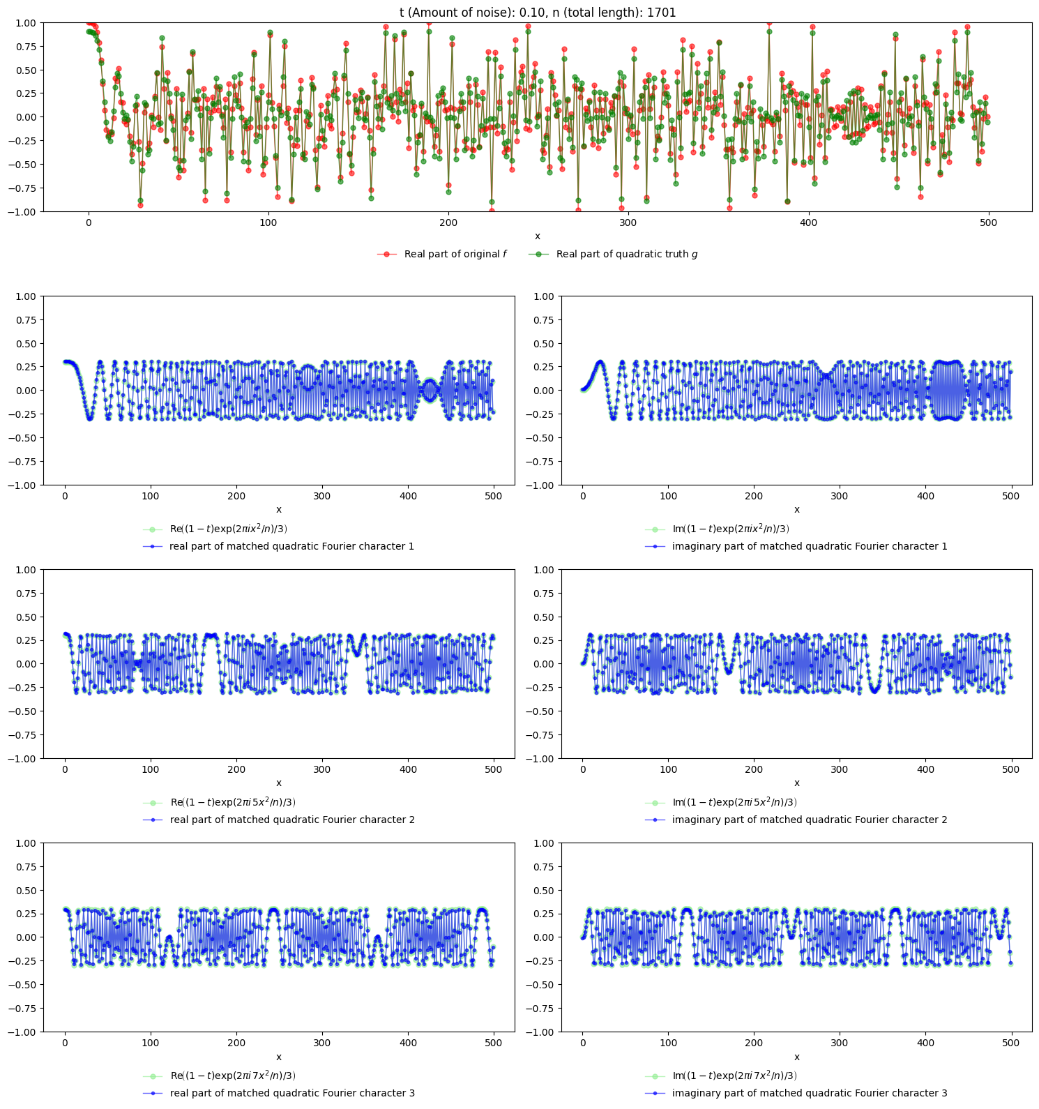
Let \(n=1701\) and consider the following function \(g:\{0,\ldots,n-1\}\to \mathbb{C}\) given by
We would like to obtain the higher-order Fourier characters of \(g\). As usual, suppose that, for \(t=0.1\), instead of \(g\) we are presented with a noisy version \(f(x)=(1-t)g(x)+tf_r(x)\), except that now \(f_r(x)= \exp(2\pi i x^3/n)\), i.e. not a uniformly random noise, but rather a polynomial phase function of order greater than 2. Note that, even though \(f_r\) is also a polynomial wave, the fact that it has a higher degree implies that it should be regarded as noise for the purposes of quadratic regularization.
n = 1701
t = 0.1

x = np.arange(n)
g = np.exp(2 * np.pi * 1j * x**2 / n) + np.exp(2 * np.pi * 5 * 1j * x**2 / n) + np.exp(2 * np.pi * 7 * 1j * x**2 / n)

f = np.exp(2 * np.pi * 1j * x**3 / n)*t+(1-t)*g/3
Objective#
To recover the individual quadratic characters that make up \(g\).
Strategy#
Simply apply hofa.char.spechoft.
rnd_sep_result = char.spechoft(f, rng=28)

eichars = rnd_sep_result.higher_order_char
import itertools
import numpy as np
import matplotlib.pyplot as plt

number_of_first_elems_to_plot = 500

v_1 = eichars[:, -1]
coeff_proj_1 = np.mean(f * v_1.conjugate())

v_2 = eichars[:, -2]
coeff_proj_2 = np.mean(f * v_2.conjugate())

v_3 = eichars[:, -3]
coeff_proj_3 = np.mean(f * v_3.conjugate())

# Restrict to plotting window
x_plot = x[:number_of_first_elems_to_plot]

# Target ("green") complex curves
target_1_complex = (1 - t) * np.exp(2 * np.pi * 1j * x_plot**2 / n) / 3
target_2_complex = (1 - t) * np.exp(2 * np.pi * 5 * 1j * x_plot**2 / n) / 3
target_3_complex = (1 - t) * np.exp(2 * np.pi * 7 * 1j * x_plot**2 / n) / 3

targets_complex = [target_1_complex, target_2_complex, target_3_complex]

# Recovered ("blue") complex curves
blue_1_complex = coeff_proj_1 * v_1[:number_of_first_elems_to_plot]
blue_2_complex = coeff_proj_2 * v_2[:number_of_first_elems_to_plot]
blue_3_complex = coeff_proj_3 * v_3[:number_of_first_elems_to_plot]

blues_complex = [blue_1_complex, blue_2_complex, blue_3_complex]

# --- L^2 (squared) error comparison over all 3! possible assignments ---
# Match using the full complex-valued curves

best_perm = None
best_err = np.inf

for perm in itertools.permutations(range(3)):
    total_err = sum(
        np.sum(np.abs(blues_complex[perm[i]] - targets_complex[i])**2)
        for i in range(3)
    )
    if total_err < best_err:
        best_err = total_err
        best_perm = perm

# Reorder blues according to best assignment
matched_blues_complex = [blues_complex[best_perm[i]] for i in range(3)]

# Labels
target_labels_real = [
    r'$\mathrm{Re}\!\left((1-t)\exp(2\pi i x^2/n)/3\right)$',
    r'$\mathrm{Re}\!\left((1-t)\exp(2\pi i\,5x^2/n)/3\right)$',
    r'$\mathrm{Re}\!\left((1-t)\exp(2\pi i\,7x^2/n)/3\right)$',
]

target_labels_imag = [
    r'$\mathrm{Im}\!\left((1-t)\exp(2\pi i x^2/n)/3\right)$',
    r'$\mathrm{Im}\!\left((1-t)\exp(2\pi i\,5x^2/n)/3\right)$',
    r'$\mathrm{Im}\!\left((1-t)\exp(2\pi i\,7x^2/n)/3\right)$',
]

blue_labels_real = [
    r"real part of matched quadratic Fourier character 1",
    r"real part of matched quadratic Fourier character 2",
    r"real part of matched quadratic Fourier character 3",
]

blue_labels_imag = [
    r"imaginary part of matched quadratic Fourier character 1",
    r"imaginary part of matched quadratic Fourier character 2",
    r"imaginary part of matched quadratic Fourier character 3",
]

# --- Plotting ---

# 4 rows x 2 columns:
# top row spans both columns,
# then 3 rows of 2 plots each
fig = plt.figure(figsize=(15, 16))
gs = fig.add_gridspec(4, 2, height_ratios=[1, 1, 1, 1], width_ratios=[1, 1])

# Top plot
ax_top = fig.add_subplot(gs[0, :])
ax_top.plot(
    x_plot,
    np.real(f[:number_of_first_elems_to_plot]),
    linestyle="-",
    color="red",
    marker="o",
    markersize=5,
    linewidth=1,
    alpha=0.6,
    label=r"Real part of original $f$",
)
ax_top.plot(
    x_plot,
    np.real((1 - t) * g[:number_of_first_elems_to_plot] / 3),
    linestyle="-",
    color="green",
    marker="o",
    markersize=5,
    linewidth=1,
    alpha=0.6,
    label=r"Real part of quadratic truth $g$",
)
ax_top.set_xlabel("x")
ax_top.set_title(f"t (Amount of noise): {t:.2f}, n (total length): {n}")
ax_top.set_ylim(-1, 1)
ax_top.legend(loc="upper center", bbox_to_anchor=(0.5, -0.15), ncol=2, frameon=False)

# Bottom 3x2 comparison plots
for i in range(3):
    target = targets_complex[i]
    blue = matched_blues_complex[i]

    # Left: real parts
    ax_real = fig.add_subplot(gs[i + 1, 0])
    ax_real.plot(
        x_plot,
        np.real(target),
        linestyle="-",
        color="lightgreen",
        marker="o",
        markersize=5,
        linewidth=1,
        alpha=0.6,
        label=target_labels_real[i],
    )
    ax_real.plot(
        x_plot,
        np.real(blue),
        linestyle="-",
        color="blue",
        marker="o",
        markersize=3,
        linewidth=1,
        alpha=0.6,
        label=blue_labels_real[i],
    )
    ax_real.set_xlabel("x")
    ax_real.set_ylim(-1, 1)
    ax_real.legend(loc="upper center", bbox_to_anchor=(0.5, -0.15), ncol=1, frameon=False)

    # Right: imaginary parts
    ax_imag = fig.add_subplot(gs[i + 1, 1])
    ax_imag.plot(
        x_plot,
        np.imag(target),
        linestyle="-",
        color="lightgreen",
        marker="o",
        markersize=5,
        linewidth=1,
        alpha=0.6,
        label=target_labels_imag[i],
    )
    ax_imag.plot(
        x_plot,
        np.imag(blue),
        linestyle="-",
        color="blue",
        marker="o",
        markersize=3,
        linewidth=1,
        alpha=0.6,
        label=blue_labels_imag[i],
    )
    ax_imag.set_xlabel("x")
    ax_imag.set_ylim(-1, 1)
    ax_imag.legend(loc="upper center", bbox_to_anchor=(0.5, -0.15), ncol=1, frameon=False)

fig.tight_layout()
plt.show()
Example: locating quadratic behaviour in data analysis#
The next example shows how hofa.char.spechoft can locate quadratic behaviour spatially, not only if it is given as a superposition of quadratic (or higher-order) waves.
Problem statement#
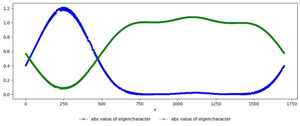
Let \(n=1701\), \(m=500\), and let us define \(f:\{0,\ldots,n-1\}\to \mathbb{C}\) as follows:
n = 1701
m = 500

x = np.arange(n)
f = np.exp(2 * np.pi * 1j * x**2 / n)
f[m:] = np.exp(2 * np.pi * 5 * 1j * x**2 / n)[m:]
Strategy#
We would like to isolate as much as we can the two components of this function.
To do so, we apply hofa.char.spechoft. This time, for illustration purposes, we add a callback function to print the advances in the iterations.
rnd_sep_result = char.spechoft(f , rng=28, callback = char.PrintRandomizedSearchCallback())

eichars = rnd_sep_result.higher_order_char
Total number of iterations 1, iterative search = True, eig vals found = 2, target num eig vals = 2
Results#
We can already see from the message above that hofa.char.spechoft was able to correctly discover that there are two very different components hiding in \(f\). First, let us print the absolute value of the higher-order characters found. Note that it clearly separates the two quadratic components.
fig, ax = plt.subplots(figsize=(12, 5))

colors = ['blue', 'green', 'yellow', 'red']

for i in range(2):
    # Plot recovered function in blue
    v = rnd_sep_result.higher_order_char[...,i]
    coeff_proj = np.mean(f*v.conjugate())
    ax.plot(x, np.abs(coeff_proj*v), linestyle='-', color=colors[i], marker='o', markersize=3, linewidth=1, alpha=0.6, label='abs value of eigencharacter')

# Customize the plot
ax.set_xlabel("x")
#ax.set_ylim(-1,1)

# Legend below the plot
fig.subplots_adjust(bottom=0.25)  # Adjust layout to fit legend below
ax.legend(loc='upper center', bbox_to_anchor=(0.5, -0.15), ncol=2, frameon=False)

# Show the plot
plt.show()
Let us plot below the different components together with the ones found by the spectral higher-order Fourier transform.
import itertools
import numpy as np
import matplotlib.pyplot as plt

number_of_first_elems_to_plot = 1000

v_1 = eichars[:, -1]
coeff_proj_1 = np.mean(f * v_1.conjugate())

v_2 = eichars[:, -2]
coeff_proj_2 = np.mean(f * v_2.conjugate())

# Restrict to plotting window
x_plot = x[:number_of_first_elems_to_plot]

# Target ("green") complex curves
target_1_complex = np.zeros_like(x_plot, dtype=complex)
target_1_complex[:m] = np.exp(2 * np.pi * 1j * x_plot**2 / n)[:m]

target_2_complex = np.zeros_like(x_plot, dtype=complex)
target_2_complex[m:] = np.exp(10 * np.pi * 1j * x_plot**2 / n)[m:]

targets_complex = [target_1_complex, target_2_complex]

# Recovered ("blue") complex curves
blue_1_complex = coeff_proj_1 * v_1[:number_of_first_elems_to_plot]
blue_2_complex = coeff_proj_2 * v_2[:number_of_first_elems_to_plot]

blues_complex = [blue_1_complex, blue_2_complex]

# --- L^2 (squared) error comparison over all possible assignments ---

best_perm = None
best_err = np.inf

for perm in itertools.permutations(range(2)):
    total_err = sum(
        np.sum(np.abs(blues_complex[perm[i]] - targets_complex[i])**2)
        for i in range(2)
    )
    if total_err < best_err:
        best_err = total_err
        best_perm = perm

# Reorder blues according to best assignment
matched_blues_complex = [blues_complex[best_perm[i]] for i in range(2)]

# Labels
target_labels_real = [
    r'$\mathrm{Re}\!\left(\exp(2\pi i x^2/n)/2i\right)$ for $x< m$',
    r'$\mathrm{Re}\!\left(\exp(10\pi ix^2/n)/2i\right)$ for $x> m$',
]

target_labels_imag = [
    r'$\mathrm{Im}\!\left(\exp(2\pi i x^2/n)/2i\right)$ for $x< m$',
    r'$\mathrm{Im}\!\left(\exp(10\pi ix^2/n)/2i\right)$ for $x> m$',
]

blue_labels_real = [
    r"real part of matched quadratic Fourier character 1",
    r"real part of matched quadratic Fourier character 2",
]

blue_labels_imag = [
    r"imaginary part of matched quadratic Fourier character 1",
    r"imaginary part of matched quadratic Fourier character 2",
]

# --- Plotting ---

fig = plt.figure(figsize=(15, 16))
gs = fig.add_gridspec(4, 2, height_ratios=[1, 1, 1, 1], width_ratios=[1, 1])

# Top plot
ax_top = fig.add_subplot(gs[0, :])
ax_top.plot(
    x_plot,
    np.real(f[:number_of_first_elems_to_plot]),
    linestyle="-",
    color="red",
    marker="o",
    markersize=5,
    linewidth=1,
    alpha=0.6,
    label=r"Real part of input $f$",
)
ax_top.set_xlabel("x")
ax_top.legend(loc="upper center", bbox_to_anchor=(0.5, -0.15), ncol=2, frameon=False)

# Bottom 3x2 comparison plots
for i in range(2):
    target = targets_complex[i]
    blue = matched_blues_complex[i]

    # Left: real parts
    ax_real = fig.add_subplot(gs[i + 1, 0])
    ax_real.plot(
        x_plot,
        np.real(target),
        linestyle="-",
        color="lightgreen",
        marker="o",
        markersize=5,
        linewidth=1,
        alpha=0.6,
        label=target_labels_real[i],
    )
    ax_real.plot(
        x_plot,
        np.real(blue),
        linestyle="-",
        color="blue",
        marker="o",
        markersize=3,
        linewidth=1,
        alpha=0.6,
        label=blue_labels_real[i],
    )
    ax_real.set_xlabel("x")
    ax_real.legend(loc="upper center", bbox_to_anchor=(0.5, -0.15), ncol=1, frameon=False)

    # Right: imaginary parts
    ax_imag = fig.add_subplot(gs[i + 1, 1])
    ax_imag.plot(
        x_plot,
        np.imag(target),
        linestyle="-",
        color="lightgreen",
        marker="o",
        markersize=5,
        linewidth=1,
        alpha=0.6,
        label=target_labels_imag[i],
    )
    ax_imag.plot(
        x_plot,
        np.imag(blue),
        linestyle="-",
        color="blue",
        marker="o",
        markersize=3,
        linewidth=1,
        alpha=0.6,
        label=blue_labels_imag[i],
    )
    ax_imag.set_xlabel("x")
    ax_imag.legend(loc="upper center", bbox_to_anchor=(0.5, -0.15), ncol=1, frameon=False)

fig.tight_layout()
plt.show()
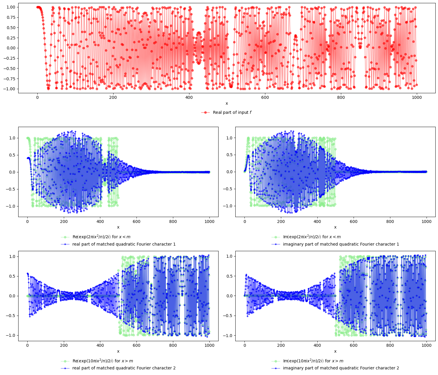
Theoretical justification#
Why is the method hofa.char.spechoft finding this spatial behaviour? The answer lies in the definition of what a quadratic Fourier character is. Recall from the U3-norm case in the Conceptual background that we defined quadratic Fourier characters as functions such that their multiplicative derivatives are (essentially) the sum of few classical Fourier characters.
The function \(f\) can be written as follows:
where \(1_A\) denotes the indicator function of a subset \(A\) of \(\{0,\ldots,n-1\}\) (that is, \(1_A(x)\) equals 1 if \(x\in A\) and 0 otherwise). In this case, \(A\) is either \([0,m]=\{x\in \{0,\ldots,n-1\}: x\le m\}\) or \((m,n)=\{x\in \{0,\ldots,n-1\}: x> m\}\).
Recall from the Important observation that a quadratic character times a function which is the sum of few Fourier characters is also a quadratic character. In this case, both \(1_{[0,m]}(x)\) and \(1_{(m,n)}(x)\) are not exactly the sum of few classical Fourier characters, but it is true that they can be approximated very well by the sum of few classical Fourier characters. Hence, under the lens of the function hofa.char.spechoft, both \(\exp(2\pi i x^2/n) 1_{[0,m]}(x)\) and \( \exp(10\pi i x^2/n) 1_{(m,n)}(x) \) are approximately two distinct quadratic characters and their sum \(f\) is simply that: their sum! This is the reason why hofa.char.spechoft finds approximations of \(\exp(2\pi i x^2/n) 1_{[0,m]}(x)\) and \( \exp(10\pi i x^2/n) 1_{(m,n)}(x) \).