Denoising and regularization: rgz and cdf modules (Checked: D)

NOTE: This tutorial assumes familiarity with the concepts explained in Conceptual and mathematical background of higher-order Fourier analysis and that the HoFa package has already been installed, see Installation.

HOW TO READ THIS NOTEBOOK: This notebook starts from a simplified version of the algorithm and progressively introduces the full generality of the implementation. Readers interested only in usage may skip to How the algorithm is implemented in practice, while readers interested in design choices may follow the full narrative.

In this notebook we are going learn how the HoFa package removes \(U^k\) noise from a function, and we are going to explain the implementation details of the regularization algorithm.

The algorithm: a minimal but representative formulation

We begin by presenting the algorithm in a deliberately restricted form. This version captures the full logical structure of the method while avoiding additional choices and tunable components that, although important in practice, are not essential for understanding how the algorithm works. The general implementation provided by the package follows the same core steps and introduces further flexibility only where meaningful alternatives arise. By starting from this minimal formulation, we can focus on the underlying mechanism of the algorithm before discussing how it can be extended, customized, and optimized.

Throughout this section, it is useful to keep in mind that every component introduced here has a direct counterpart in the full implementation. Later sections will revisit each step and show how it can be modified or replaced to accommodate different variants of the algorithm.

Let us recall below with pseudocode the basic version we are interested in.

Basic \(U^3\) regularization algorithm

Input: \(f: Z \to \mathbb{C}\), \(\rho, \varepsilon {>0}\)

1. \(M \leftarrow f(x) \otimes \overline{f(y)} \in \mathbb{C}^{Z \times Z}\)

2. For each \(t \in Z\):

   • \(M(\cdot + t, \cdot) \leftarrow K_\varepsilon(M(\cdot + t, \cdot))\)

3. \((\mu_1, v_1), \ldots, (\mu_{|Z|}, v_{|Z|}) \leftarrow \mathrm{Eigdecomp}(M)\)

Output: \(f_{\text{reg}} \leftarrow\sum_{\mu_i \ge \rho} \langle f, v_i \rangle v_i\), eigenvalues \(\leftarrow \{\mu_1,\ldots, \mu_{|Z|}\}\), and eigenvectors \(\leftarrow \{v_{1},\ldots, v_{|Z|}\}\).

To better understand how the algorithm works, we now walk through its basic formulation step by step on a simple example. By explicitly computing the intermediate quantities, we expose the internal logic that is otherwise hidden by the implementation. This perspective will be useful when we later introduce more general variants of the algorithm.

Manual execution of the basic algorithm

We consider the following illustrative problem, which will serve as a running example throughout this section.

Problem statement

We want to transmit the periodic linear chirp \(f_s(x)=\sin(2\pi x^2/n)\) defined for any integer \(x\) (note the periodicity property \(f_s(x+n)=f_s(x)\)). However, our communication channel introduces noise, and what is received is a convex combination \(f=tf_r+(1-t)f_s\) where \(f_r(x)\) follows a uniform distribution \(\text{Unif}([-1,1))\) independently for every integer \(x\) and the amount of noise is \(t=30\)%.

This formulation intentionally simple and is chosen to highlight the core behavior of the algorithm rather than edge cases.

Objective

Under these assumptions, we aim to compute an estimate of \(f_s\).

In the following, we use this example to manually execute the algorithm step by step, making explicit the intermediate quantities involved in the computation.

First of all, let us import the necessary modules. Recall that we are assuming that the HoFa package is already installed, see Installation. For a quick installation, run the following command:

(hofavenv) $ pip install hofa

# Import the necessary packages to use hofa
import hofa.cdf as cdf
import hofa.rgz as rgz

# and visualize its results
import numpy as np
np.set_printoptions(precision=2)
import matplotlib.pyplot as plt
import scipy

Modelization of the example problem

Setup:

• \(f_s(x):\mathbb{Z}\to \mathbb{R}\) is defined as \(x\mapsto \sin(2\pi x^2/n)\),

• \(f_r:\mathbb{Z}\to \mathbb{R}\) is defined as \(f_r(x)\sim \text{Unif}([-1,1))\) independently for every \(x\in \mathbb{Z}\),

• \(f:=t f_r+(1-t)f_s\) for \(t=0.3\).

Goal: Recover \(f_s\) using only \(f\).

n = 173 # Feel free to change this
x = np.arange(n)
f_s = np.sin(2*np.pi*x**2/n)
# Due to implementation reasons of auxiliary functions, 
# it is convenient to work with complex numbers
f_s = f_s.astype(complex) 

# For reproducibility reasons, we fix a random seed, but feel free to change this.
np.random.seed(123)
f_r = np.random.uniform(-1, 1, size=len(x))

# And finally we construct the only function we are going to work with, f.
# To do that, we fix t=0.3, but again, feel free to change it and test the limits of the algorithm.
t = 0.3
f = t*f_r+(1-t)*f_s

The algorithm step by step

Now that we have defined our function, it is time to implement Basic \(U^3\) regularization algorithm. To do so, not that the first step is to compute \(f\otimes \overline{f}\). The module rgz provides us with the method hofa.rgz.t_prod_itself to compute such matrix.

M = rgz.t_prod_itself(f) # We compute the matrix
M[:5,:5] # And we visualize only the first 5x5 upper left corner

array([[ 0.01+0.j, -0.01-0.j, -0.01-0.j,  0.03+0.j,  0.06+0.j],
       [-0.01+0.j,  0.01+0.j,  0.01+0.j, -0.03+0.j, -0.05+0.j],
       [-0.01+0.j,  0.01+0.j,  0.  +0.j, -0.02+0.j, -0.03+0.j],
       [ 0.03+0.j, -0.03-0.j, -0.02-0.j,  0.07+0.j,  0.13+0.j],
       [ 0.06+0.j, -0.05-0.j, -0.03-0.j,  0.13+0.j,  0.27+0.j]])

We see that the result is a real symmetric matrix \(M_{n\times n}(\mathbb{R})\). In general, if the map \(f\) takes complex values then the resulting matrix will be self-adjoint.

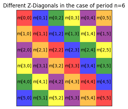
The second step in Basic \(U^3\) regularization algorithm consists in changing the \(Z\)-diagonals of \(M\) for a Fourier regularized version. Note that the \(Z\)-diagonals are not the usual diagonals of a matrix as they are defined using modular arithmetic. That is, if \(M=(m_{i,j})_{i,j=0,\ldots,n-1}\) , a \(Z\)-diagonal of height \(t=0,\ldots,n-1\) a collection of \(m_{i,j}\) are in the same diagonal if \(i-j\) equal the same integer \(t\) modulo \(n\). This part is important, so let us draw a diagram where we highlight the different diagonals. For simplicity, imagine now that \(n=6\) instead of \(n=173\) as we have above. Thus, the matrix \(M\) is 6x6 and its \(Z\)-diagonals are as follows.

from matplotlib.colors import ListedColormap, BoundaryNorm

matrix = np.array([
    [0, 1, 2, 3, 4, 5],
    [5, 0, 1, 2, 3, 4],
    [4, 5, 0, 1, 2, 3],
    [3, 4, 5, 0, 1, 2],
    [2, 3, 4, 5, 0, 1],
    [1, 2, 3, 4, 5, 0]
])

colors = ["red", "blue", "green", "yellow", "purple", "orange"]

cmap = ListedColormap(colors)
norm = BoundaryNorm(np.arange(-0.5, 6.5, 1), cmap.N)

plt.figure(figsize=(4, 4))
plt.imshow(matrix, cmap=cmap, norm=norm, alpha=0.7)
plt.xticks([])
plt.yticks([])

for i in range(6):
    for j in range(6):
        plt.text(j, i, 'm['+str(i)+','+str(j)+']',
                 ha="center", va="center", color="black")

plt.title('Different Z-Diagonals in the case of period n=6')
plt.show()

There are many ways of operating on the \(Z\)-diagonals of a matriz but currently, there are no fast numpy or scipy method that can vectorize an operation through them. The solution given in hofa.rgz is to create an auxiliary matrix where the \(Z\)-diagonals of a function are moved to the rows using hofa.rgz.move_diag_to_rows so that we can operate with them easily, and then a function to put them back in their original positions hofa.rgz.move_rows_to_diag. Let us see in action how these methods in action on our toy example:

M_diag_to_rows = rgz.move_diag_to_rows(M)
M_diag_to_rows[:5,:5]

array([[ 0.01+0.j,  0.01+0.j,  0.  +0.j,  0.07+0.j,  0.27+0.j],
       [-0.01-0.j,  0.01+0.j, -0.02+0.j,  0.13+0.j,  0.26+0.j],
       [-0.01-0.j, -0.03+0.j, -0.03+0.j,  0.13+0.j,  0.5 +0.j],
       [ 0.03+0.j, -0.05+0.j, -0.03+0.j,  0.25+0.j,  0.41+0.j],
       [ 0.06+0.j, -0.05+0.j, -0.06+0.j,  0.2 +0.j,  0.26+0.j]])

Note that, e.g., the main diagonal is now the first row in the M_diag_to_rows matrix.

To put it back to its original state, we can use hofa.rgz.move_rows_to_diag.

M_back_to_position = rgz.move_rows_to_diag(M_diag_to_rows)
print(f" All elements correctly reorganized: {np.all(M == M_back_to_position)}")

 All elements correctly reorganized: True

The actual implementation of both these functions currently use Broadcasting and Advanced indexing to handle not only the case of 1-dimensional \(n\)-periodic function but also the general case of any number of dimensions with different periods, see Coding theory example.

But remember that what we want is to create a new matrix where we have changed the \(Z\)-diagonals by applying the Denoising operator \(K_\varepsilon\), see Basic \(U^3\) regularization algorithm. Remember that this operator uses a small constant \(\varepsilon\) defined by the user, so let us fix one such constant and define the denoising operator \(K_\varepsilon\).

epsilon = 0.03

def denoising_operator(diag : np.ndarray):
    """
    Modifies the function `diag` on the finite abelian group Z to produce K_epsilon(diag).

    Parameters:
        diag (function): The function defined on Z.

    Returns:
        function: The modified function K_epsilon(diag).
    """
    # Compute all Fourier coefficients of diag
    fourier_coeffs = np.fft.fftn(diag,norm="forward")

    # Modify Fourier coefficients as per the algorithm
    modified_coeffs = (np.maximum(np.abs(fourier_coeffs)-epsilon,0))*np.exp(1j*np.angle(fourier_coeffs))

    # Return the new function K_epsilon(diag) using the modified Fourier coefficients
    return np.fft.ifftn(modified_coeffs, norm="forward")

Now, we need to apply this operator on every \(Z\)-diagonal of our \(Z\)-matrix \(M\). To do so, we have the method hofa.rgz.apply_on_diag. This method essentially uses hofa.rgz.move_diag_to_rows to put all diagonals as rows, applies an operator to each diagonal, and puts the diagonals back in their original places with hofa.rgz.move_rows_to_diag.

Note: This is one of the places where performance could be enhanced by providing native methods written in C for handling \(Z\)-diagonals. Note that this process of applying an operator on every \(Z\)-diagonal can be parallelized, as we will see in the appropriate tutorial where we deal with the PyTorch implementation.

M_diags_reg = rgz.apply_on_diag(M, denoising_operator)

# Similarly as before, we compute the same for our toy example M_g
M_g_diags_reg = rgz.apply_on_diag(M, denoising_operator)
M_g_diags_reg[:4,:4]

array([[0.21+2.78e-17j, 0.22-1.39e-17j, 0.21+6.94e-18j, 0.2 -2.78e-17j],
       [0.22+7.98e-17j, 0.24+9.45e-17j, 0.22+6.25e-17j, 0.21-5.20e-17j],
       [0.21+5.38e-17j, 0.22-6.25e-17j, 0.25-6.94e-18j, 0.21-4.16e-17j],
       [0.2 -1.39e-17j, 0.21+1.18e-16j, 0.21+4.86e-17j, 0.26-4.16e-17j]])

After this strange-looking operation we are ready to see where the magic starts. Precisely, we need now to compute the eigendecomposition of \(M\).

Note: We prefer to use a different normalization for eigenvalues and eigenvectors other than the one of np.linalg.eigh. The reason is that if we treat \(M\) as a kernel operator, we should normalize the application of \(M\) on a vector dividing by the length of the vector. That is, as a kernel operator \(M\) applied on a vector \(v\) should be defined as \(\tfrac{1}{n}Mv\). This is consistent with e.g. normalizing the forward Fourier transform \(\widehat{f}(\chi)=\tfrac{1}{n}\sum_{x=0}^{n-1} f(x)\overline{\chi(x)}\) as we always do in the HoFa package. In practive this means that we have to divide the eigenvalues resulting from np.linalg.eigh by \(n\) and multiply the eigenvectors by \(\sqrt{n}\) (so that they have norm 1 when we compute the normalized \(L^2\) norm \(\|f\|_2^2=\tfrac{1}{N}\sum_{x=0}^{n-1} |f(x)|^2\)).

eivals, eivects = np.linalg.eigh(M_diags_reg)

# To normalize eigenvalues and eigenvectors we need to do
# the following
eivals = eivals/n
eivects = eivects*np.sqrt(n)

The magic here occurs when we look at the eigenvalues of M_diags_reg. Recall that these are ordered increasingly.

plt.figure(figsize=(3, 2))
plt.plot(eivals, marker='o', linestyle='None')
plt.show()

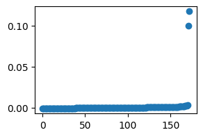
Note that there is something strange here, there two eigenvalues whose absolute value is significantly greater than the rest. The deep reason for this is that, with respect to this algorithm, we are seeing our function \(f_s(x)=\sin(2\pi x^2/n)\) as a combination of two higher-order characters

\[\sin(2\pi x^2/n) = \frac{e^{2\pi i x^2/n}-e^{-2\pi i x^2/n}}{2i}.\]

Note: that we have computed this using only \(f=tf_r+(1-t)f_s\), the algorithm has not seen \(f_s\) but nevertheless it has been able to recognize not only the quadratic structure, but also the fact that it comes from 2 higher-order characters.

Our Basic \(U^3\) regularization algorithm tells us that projecting the function \(f\) to the eigenspace generated by the eigenvectors corresponding to these two eigenvalues keeps precisely the quadratic component of the function \(f\).

# Now we compute the projection of f on that eigenvector
f_reg = np.mean(f*eivects[:,-1].conjugate())*eivects[:,-1]+np.mean(f*eivects[:,-2].conjugate())*eivects[:,-2]

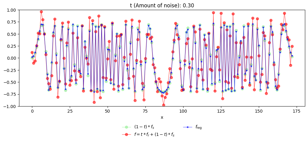
And to conclude let us plot this function together with the original function \(f\) that we feeded the algorithm with and the real quadratic component \((1-t)f_s\) that is hidden within \(f\).

# And now let us print the original function f_s*(1-t), the modified version
# f, and the output of our algorithm f_reg. (For simplicity we only plot
# the real part of those functions).
fig, ax = plt.subplots(figsize=(12, 5))

# Plot original (1-t)*f_s in light green
ax.plot(x, np.real(f_s*(1-t)), linestyle='-', color='lightgreen', marker='o', markersize=6, linewidth=1, alpha=0.6, label=r'$(1-t)*f_s$')

# Plot modified function in red
ax.plot(x, np.real(f), linestyle='-', color='red', marker='o', markersize=6, linewidth=1, alpha=0.6, label=r'$f = t*f_r+(1-t)*f_s$')

# Plot recovered function in blue
ax.plot(x, np.real(f_reg), linestyle='-', color='blue', marker='o', markersize=3, linewidth=1, alpha=0.6, label=r'$f_{\text{reg}}$')

# Customize the plot
ax.set_xlabel("x")
ax.set_title(f"t (Amount of noise): {t:.2f}")
ax.set_ylim(-1,1)

# Legend below the plot
fig.subplots_adjust(bottom=0.25)  # Adjust layout to fit legend below
ax.legend(loc='upper center', bbox_to_anchor=(0.5, -0.15), ncol=2, frameon=False)

# Show the plot
plt.show()

Before continue, the reader is encouraged to modify the above example with different functions, parameters \(\varepsilon,\rho, t, n\) etc.

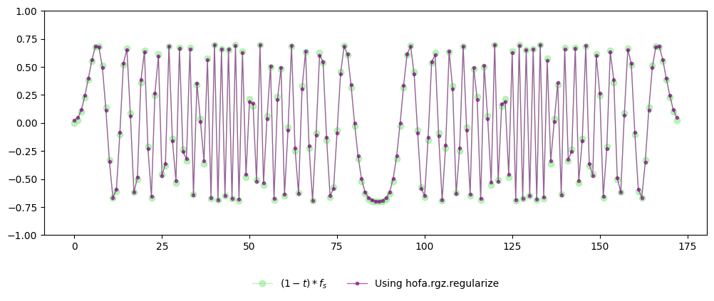
The sequence of operations we have just carried out manually is exactly what the package implements internally. In practice, all of the steps above are encapsulated in a single function call to hofa.rgz.regularize(), which performs the same computation while handling the necessary bookkeeping and numerical details. Moreover, it includes heuristics to compute the parameters \(\varepsilon,\rho\).

fig, ax = plt.subplots(figsize=(12, 5))

ax.plot(x, np.real(f_s*(1-t)), linestyle='-', color='lightgreen', marker='o', markersize=6, linewidth=1, alpha=0.6, label=r'$(1-t)*f_s$')

ax.plot(x, np.real(rgz.regularize(f,2).regularization), linestyle='-', color='purple', marker='o', markersize=3, linewidth=1, alpha=0.6, label=r'Using hofa.rgz.regularize')

ax.set_ylim(-1,1)
fig.subplots_adjust(bottom=0.25)  # Adjust layout to fit legend below
ax.legend(loc='upper center', bbox_to_anchor=(0.5, -0.15), ncol=2, frameon=False)

plt.show()

Generalizing the algorithm

While the basic formulation already captures the core idea of the algorithm, it is not the only reasonable way to instantiate it. Several aspects of the procedure admit alternative choices, leading to variants that differ in behavior, robustness, or computational cost. The package is designed to expose these degrees of freedom in a controlled way, allowing users to adapt the algorithm to specific problems while preserving the underlying structure described above. Let us now discuss where these alternatives may take place by pinpointing in the Basic \(U^3\) regularization algorithm possible variants.

Input: \(f: Z \to \mathbb{C}\), \(\rho, \varepsilon {>0}\) → 1

1. \(M \leftarrow f(x) \otimes \overline{f(y)} \in \mathbb{C}^{Z \times Z}\)

2. For each \(t \in Z\):

   • \(M(\cdot + t, \cdot) \leftarrow K_\varepsilon(M(\cdot + t, \cdot))\) → 2

3. \((\mu_1, v_1), \ldots, (\mu_{|Z|}, v_{|Z|}) \leftarrow \mathrm{Eigdecomp}(M)\) → 3

Output: \(f_{\text{reg}} \leftarrow\sum_{\mu_i \ge \rho} \langle f, v_i \rangle v_i\), eigenvalues \(\leftarrow \{\mu_1,\ldots, \mu_{|Z|}\}\), and eigenvectors \(\leftarrow \{v_{1},\ldots, v_{|Z|}\}\).

→ 1 How can we choose these parameters \(\varepsilon\) and \(\rho\)?

→ 2 So far we used the map denoising_operator for regularizing the diagonals, which changes any diagonal \(g \mapsto \sum \mathrm{ReLU}(|\widehat{g}(\chi)|-\varepsilon)\tfrac{\widehat{g}(\chi)}{|\widehat{g}(\chi)|}\chi\). But can we use other method such as simply \(g \mapsto \sum_{|\widehat{g}(\chi)|\ge \varepsilon}\widehat{g}(\chi)\chi\) ? and moreover, what if we want to do cubic or higher-order regularization? As explained in Order increment principle, page 4, Figure 1 we should replace \(K_\varepsilon\) with a lower order regularizer. For instance, if we want cubic regularization we should replace \(K_\varepsilon\) with the Basic \(U^3\) regularization algorithm itself!

→ 3 Last but not least, we have to compute the eigendecomposition of a matrix. But we are typically interested only in the largest eigenvalues and eigenvectors. Moreover, the size of the largest eigenvalues needed depend on this last cutoff parameter \(\rho\). Hence, in general we do not want to compute the full eigendecomposition using numpy.linalg.eigh, is there anything better?

All these question will be adressed below, where we will see how to precisely handle all of these issues.

How the algorithm is implemented in practice

So far, we have explored the basic version of the algorithm and walked through its steps manually to build intuition. The version implemented in the package follows the same core logic but adds flexibility and tunable components that allow it to handle a wider range of practical scenarios.

Let us now present the full algorithm in pseudocode and explain how its different parts are implemented. We start with the main function that encapsulates the internal logic, then describe auxiliary functions and classes that provide additional control for advanced users.

To understand this pseudocode, recall that this is a recursive algorithm. Let us denote by \(K(f,k)\) its output for a function \(f\) if we want regularization of order \(k\).

General \(U^k\) regularization algorithm

Input: Function to regularize: \(f: Z \to \mathbb{C}\) and order of regularization: \(k\) (a positive integer)

0. If \(k==1\):

   Output: \(K(f,1)\): Fourier regularization on \(f\), absolute value squared of Fourier coefficients \(|\widehat{f}(\chi)|^2\), and all Fourier characters \(\{\chi\}\).

1. \(M \leftarrow f(x) \otimes \overline{f(y)} \in \mathbb{C}^{Z \times Z}\)

2. For each \(t \in Z\):

   • Replace the \(Z\)-diagonal \(M(\cdot + t, \cdot)\) in the \(Z\)-diagonal with the \(k-1\)-regularized version \(K((M(\cdot + t, \cdot),k-1)\).

3. \((\mu_1, v_1), \ldots, (\mu_{|Z|}, v_{|Z|}) \leftarrow \mathrm{Eigdecomp}(M)\)

Output \(K(f,k)\): is the weighted projection of \(f\) in terms of the \(\mu_i\) to the eigenspaces \(v_i\), the eigenvalues \(\{\mu_i\}\), and the eigenvectors \(\{v_i\}\).

The pseudocode above captures the logical flow of the full algorithm, highlighting its core steps and optional variant points. Each step corresponds directly to one or more functions or classes in the package, with the main workflow implemented in the regularize() function.

# In the module hofa.rgz
def regularize(f : np.ndarray, per_layer_regularizers : List[LayerRegularizer] | int = 2, rng : int | np.random.Generator | None = None) -> RegularizationResult:

The signature of this function reflects the flexibility illustrated in the pseudocode: it accepts both simple parameters for standard usage and objects that encapsulate specific algorithmic variants, allowing advanced users to control individual steps. In other words, the main function is a direct, ready-to-use realization of the algorithm, where each argument corresponds to a concept from the pseudocode:

• Core input: the function f.

• Regularization component: the variable per_layer_regularizers which represent either an int for default regularization of some order or a List[LayerRegularizer] to allow flexibility and fine-tunning of the regularization process.

• Output: final result of the algorithm.

Exploring auxiliary functions

While the regularize() function serves as the main entry point, its role is primarily to perform setup, validate inputs, and orchestrate the overall workflow. The actual computations and algorithmic decisions are carried out by a set of auxiliary functions that implement the core steps highlighted in the pseudocode, the most important ones being:

# In the module hofa.rgz
def regularize_after_setup(f : np.ndarray, per_layer_regularizers : List[LayerRegularizer])

def regularize_and_decompose(f : np.ndarray, K : Callable , layer_regularizer : LayerRegularizer)

The function regularize_after_setup() is in charge of doing the main recursion step, while regularize_and_decompose() implements steps 1., 2., and 3. of the General \(U^k\) regularization algorithm.

Beyond these core functions, the implementation is decomposed into several smaller auxiliary functions that correspond to individual steps or sub-steps of the algorithm. This decomposition serves two purposes: it keeps the main logic readable and maintainable, and it allows advanced users to inspect or customize specific operations in isolation.

In typical usage, these auxiliary functions are invoked internally by the core functions and do not need to be called directly. Nevertheless, they are exposed as part of the public API to facilitate experimentation, debugging, or fine-grained control over specific stages of the algorithm.

Auxiliary functions

The following auxiliary functions implement individual steps of the algorithm and are primarily intended for advanced usage:

# In the module hofa.rgz
def weighed_projection(f : np.ndarray, eigvals : np.ndarray, eigvects : np.ndarray, layer_regularizer : LayerRegularizer)

• Implements the Output step of the algorithm where we need to compute the projection of a function to certain eigenspaces weighted by some parameters which depends on the eigenvalues

# In the module hofa.rgz
def default_reg_list(k : int)

• Gives a list of default tested LayerRegularizer s of a certain length.

# In the module hofa.rgz
def move_diag_to_rows(M : np.ndarray)

• Auxiliary function that re-organizes the \(Z\)-diagonals of a matrix into rows

# In the module hofa.rgz
def move_rows_to_diag(M : np.ndarray)

• Auxiliary function that re-organizes the rows of a matrix as \(Z\)-diagonals. Inverse operation of move_diag_to_rows.

# In the module hofa.rgz
def apply_on_diag(M : np.ndarray , K : Callable)

• Function to apply a certain operator into the \(Z\)-diagonals of a matrix.

# In the module hofa.rgz
def t_prod_itself(g : np.ndarray)

• Function to apply create, from a function, the corresponding matrix of step 1. of General \(U^k\) regularization algorithm.

Each of these functions is called internally by the core workflow, but can also be used independently to customize or extend specific stages of the algorithm.

Encapsulating fine-tuning and algorithmic variants

To support fine-grained control over the algorithm, the package introduces an abstract base class LayerRegularizer that defines the common interface and encapsulates the choices and behaviors that may vary between different algorithmic variants. This abstract class appears throughout the functions presented above. Rather than hard-coding specific choices into each function, the algorithm delegates these decisions to the particular implementations of such class, allowing the same workflow to support multiple variants, tuning strategies, and extensions in a consistent and modular way.

For most users, the default concrete implementation StandardLayerRegularizer provided by the package is sufficient and can be used directly without modification. Advanced users, however, may subclass the abstract class to customize specific aspects of the algorithm while preserving compatibility with the rest of the pipeline.

Finally, there is the class RegularizationResult which is nothing but a NamedTuple containing the result of the main regularization algorithm. Its signature is as follows:

class RegularizationResult(NamedTuple):
    regularization : np.ndarray
    eigenvalues : np.ndarray
    eigenvectors : np.ndarray

As the General \(U^k\) regularization algorithm is recursive in nature, note that we may want different behaviour at different heights. For instance, we may want to use a faster method for computing eigendecomposition of matrices when we have to repeat that operation many times, but we may want a more precise one when we are at a higher level and the computing time will not be affected much. This is why hofa.rgz.regularize() takes as a value a List[LayerRegularizer]. Note that the length of such list of LayerRegularizer will determine the order of regularization of the algorithm.

Before examining the concrete implementations, it is helpful to step back and look at how the abstract class fits into the overall structure of the algorithm.

The diagram below illustrates the role of the abstract class as a mediator between the high-level workflow and the low-level algorithmic choices. Rather than embedding variant-specific logic directly into each function, the algorithm delegates these decisions to an object that implements a common interface. This design allows the same core workflow to support multiple behaviors while remaining easy to extend and reason about.

The accompanying example walks through a simplified execution of the algorithm and highlights when and how the abstract class is queried during the process.

Interaction between workflow and variant logic

In the next diagram we are going to see the main workflow of a call to regularize and how the different LayerRegularizers provide the variant-specific behavior required at each decision point. To best illustrate this, let us consider the case of cubic regularization (i.e. for the \(U^4\) norm). Hence per_layer_regularizers is a List[LayerRegularizer] with len(per_layer_regularizers) equal to 3.

hofa.rgz.regularize(f , [per_layer_regularizers[0], 
                         per_layer_regularizers[1], 
                         per_layer_regularizers[2]])

The steps that we need to follow to understand this diagram are marked with blue numbers.

Function	Operator	Regularizer
1. \(f\)	2. \(f\otimes \overline{f} = \begin{pmatrix}\ddots & & \\& \Delta_t f & \\& & \ddots\end{pmatrix}\)	9. per_layer_regularizers[2]
3. \(\Delta_tf\) for each \(t\in Z\)	4. \(\Delta_tf\otimes \overline{\Delta_tf} = \begin{pmatrix}\ddots & & \\& \Delta_{t'}\Delta_t f & \\& & \ddots\end{pmatrix}\)	8. per_layer_regularizers[1]
5. \(\Delta_{t'}\Delta_tf\) for \(t,t'\in Z\)	6. No need of creating an operator, its eigenvectors are the Fourier characters and its eigenvalues are \(\vert\widehat{\Delta_{t'}\Delta_tf}(\chi)\vert^2\) for \(\chi\in\widehat{Z}\).	7. per_layer_regularizers[0]

1. We begin with the function \(f\) to do cubic regularization.

2. We construct the matrix \(f\otimes \overline{f}\).

3. For each \(Z\)-diagonal of \(f\otimes \overline{f}\), which corresponds to the function \(\Delta_tf\),

4. we construct the matrix \(\Delta_tf\otimes \overline{\Delta_tf}\).

5. For each \(Z\)-diagonal of \(\Delta_tf\otimes \overline{\Delta_tf}\), which corresponds to the function \(\Delta_{t'}\Delta_tf\),

6. we compute its Fourier regularization. We do not need to construct the matrix \(\Delta_{t'}\Delta_tf\otimes \overline{\Delta_{t'}\Delta_tf}\) as we already known that in this case we can take as eigenvalues the set \(\{|\widehat{\Delta_{t'}\Delta_tf}(\chi)|^2\}_{\chi\in\widehat{Z}}\) and \(\widehat{Z}\) as the set of eigenvectors.

7. The object per_layer_regularizers[0] will be in charge of performing the Fourier regularization for each of the \(\Delta_{t'}\Delta_t f\) functions. Thus, it will be feeded with functions of the form \(\Delta_{t'}\Delta_t f\) and it will have to return a Fourier-regularize version of them. Note that it would be convenient that per_layer_regularizers[0] has access at some point to \(\Delta_t f\) and \(f\), i.e., to the function whose multiplicative derivatives result in the function that per_layer_regularizers[0] has to regularize.

8. After per_layer_regularizers[0] has regularized all diagonals of the matrix \(\Delta_t f(x)\otimes \overline{\Delta_t f(x)}\) from step 4., the algorithm must then decompose the resulting matrix. Let us denote this regularized matrix as \(\mathcal{K}(\Delta_t f(x)\otimes \overline{\Delta_t f(x)},1)\). The object per_layer_regularizers[1] is in charge of controlling this process for each of the \(\Delta_t f(x)\), i.e., deciding which eigendecomposition method to use for \(\mathcal{K}(\Delta_t f(x)\otimes \overline{\Delta_t f(x)},1)\) and how to project to the different eigenspaces the functions \(\Delta_t f(x)\) according to some weights. Again, it would be useful if per_layer_regularizers[1] had access to \(f\).

9. After all diagonals of the matrix from step 2. are regularized, we have a matrix which we denote by \(\mathcal{K}(f(x)\otimes \overline{ f(x)},2)\). Then the object per_layer_regularizers[2] is in charge of computing the eigendecomposition of \(\mathcal{K}(f(x)\otimes \overline{ f(x)},2)\) and to then project \(f\) to the corresponding eigenspaces according to some weights which depend on the corresponding eigenvalues.

Therefore, we saw that each (implementation of) LayerRegularizer will perform a certain regularization based on its relative position position in the list per_layer_regularizers. That is, it will have to compute eigenvalues and eigenvectors of a certain matrix and then it will have to compute the weights of the different eigenspaces. Moreover, it would be convenient that each regularizer has access not only to the function to regularize, e.g. \(\Delta_{t'}\Delta_t f\) for per_layer_regularizers[0], but also to all the functions whose multiplicative derivatives used in the computation of that function, i.e., \(\Delta_t f\) and \(f\) for per_layer_regularizers[0].

Abstract class LayerRegularizer

We are now ready to understand the abstract class LayerRegularizer and how its implementation affect the execution of the regularize function.

# In hofa.rgz
class LayerRegularizer(ABC):
    
    @abstractmethod
    def __init__(self):
        pass

    @abstractmethod
    def setup(self, f : np.ndarray, depth : int, layer : int):
        pass

    @abstractmethod
    def update(self, f : np.ndarray, height : int):
        pass

    @abstractmethod
    def alpha(self, eigs : np.ndarray):
        pass

    @abstractmethod
    def eigh(self, M : np.ndarray):
        pass

Let us now explain each of those methods in depth.

Constructor

def __init__(self):

The constructor. It can have a different signature to accept parameters in order to define several version of similar implementations of LayerRegularizer.

Setup method

def setup(self, f : np.ndarray, depth : int, layer : int):

This method will be called once for each regularizer at the begining of the regularization process. The variable f is the function to regularize, depth=k represents that we want to regularize f for the \(U^{k+1}\) norm, and layer represents the position of this regularizer in the regularization process. That is, layer will be a number between \(0\) and \(k-1\). If layer=0 it means that this regularizer will do the role of Fourier regularizer (step 7. above in case for \(k=3\)), layer=1 means that it will do \(U^3\) regularization, etc.

Update

def update(self, f : np.ndarray, height : int):

This method will be called once per multiplicative derivative that sits above the one that a particular regularizer has to handle. For example, per_layer_regularizers[0] in the above example will be called with

• per_layer_regularizers[0].update(\(f\), 3),

• per_layer_regularizers[0].update(\(\Delta_t f\), 2), and finally

• per_layer_regularizers[0].update(\(\Delta_{t'}\Delta_t f\), 1)

before it has to regularize the function \(\Delta_{t'}\Delta_t f\). In between, it may be receive different calls to update but it can be certain that by the time per_layer_regularizers[0] has to regularize \(\Delta_{t'}\Delta_t f\), the latest times update was called with height equal to 1,2,3 are precisely calls corresponding to the multiplicative derivatives that sit above the particular function to regularize. These calls may be used to update internal states of per_layer_regularizers[0] in order to perform the regularization.

In general, if a particular LayerRegularizer was called in setup with depth=\(k\) and layer=\(l\), it will be called once with update(\(f\),\(k\)), \(|Z|\) times with update(\(\Delta_t f\), \(k-1\)),…, and \(|Z|^{k-l-1}\) times with update(\(\Delta_{t_1}\cdots\Delta_{t_{k-l-1}}f\), \(l\)). It is guaranteed that by the time a particular LayerRegularizer has to regularize \(\Delta_{t_1}\cdots\Delta_{t_{k-l-1}}f\), the last calls to update with the sequence of numbers \(\{k,k-1,\ldots,l\}\) in the second argument contains exactly the multiplicative derivatives that were used to create \(\Delta_{t_1}\cdots\Delta_{t_{k-l-1}}f\). This can be used to boost efficiency as typically we do not need to keep in memory all multplicative derivatives.

Eigendecomposition

def eigh(self, M : np.ndarray):

Consider the case of per_layer_regularizers[2] from the above diagram. Note that after regularizing all the diagonals of the matrix \(f\otimes \overline{f}\), we need first to compute its eigendecomposition. As later per_layer_regularizers[2] will apply some weights on the different eigenspaces, it makes no sense that it computes the full eigendecomposition. Thus, the user is allowed to program here a method that computes only the largest eigenvalues and eigenvectors that will be used later.

The case of per_layer_regularizers[0] is special as this method will be ignored. Remember that we know that a valid eigendecomposotion in the case of the \(U^2\) norm can be computed using the Fourier transform. Hence, the Fast Fourier Transform is used in this case.

The weighting function

def alpha(self, eigs : np.ndarray):

This is the method for computing the weights of the different eigenspaces. Those weigths will be used with the eigenvalues and eigenvectors of LayerRegularizer.eigh in order to regularize a function by projecting to the appropriate eigenspaces. Note that in the case of per_layer_regularizers[0] the variable eigs in the call of alpha will be the squared modules of the Fourier coefficients of the function to regularize.

Default implementation: StandardLayerRegularizer

Having defined the abstract interface LayerRegularizer, we now turn to the default concrete implementation StandardLayerRegularizer provided by the package. This implementation realizes a commonly useful variant of the algorithm and serves both as a practical, ready-to-use component and as a reference for understanding how the abstract methods are intended to be implemented.

The default use of regularize use this class, so users can benefit from the full algorithmic capabilities without interacting directly with the abstract class LayerRegularizer. At the same time, the structure of this implementation illustrates how fine-tuning and variant-specific behavior are encapsulated, making it a useful starting point for users who wish to extend or customize the algorithm.

# In hofa.rgz
class StandardLayerRegularizer(Regularizer):
    
    def __init__(self, 
                 alpha_method : Callable = hofa.cdf.relu ,  
                 param : float | int = 1.2,  
                 mode : str = 'dynamic-original', 
                 lin_alg_method : str = 'sparse',
                 num_eigen : str | int = 'dynamic'
                ):
    ...
                

The alpha_method parameter

The first argument in this constructor is alpha_method, that tells StandardLayerRegularizer which function it has to apply to the eigenvalues of the regularized matrix. Recall that each Regularizer is in charge of regularizing a particular type of function depending on its layer (given via the setup method). In most cases, for a function \(g\) (in the above example this would be either \(f\), \(\Delta_t f\), or \(\Delta_{t'}\Delta_t f\) depending on whether layer equals 2, 1, or 0 respectively) this method will compute a series of eigenvalues and eigenvectors and it will have to return a weighted projection of \(g\) to the eigenspaces weighted by some function. Recall that in case layer=0, the eigenvalues will be \(\{|\widehat{g}(\chi)|^2\}_{\chi\in \widehat{Z}}\) and the eigenvectors the set \(\widehat{Z}\).

The way StandardLayerRegularizer computes the weights of the eigenspaces depending on the eigenvalues is by applying the alpha_method given in the constructor of StandardLayerRegularizer together with a parameter \(\tau>0\). Below we explain how this parameter is computed. It is mandatory that the method given in the constructor of StandardLayerRegularizer has precisely the signature

def alpha_method(eigvals : np.ndarray, tau : int | float)

The cdf module

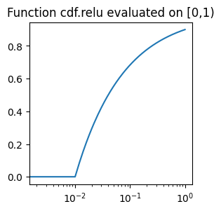
The hofa package comes with a pre-defined set of functions that can act as regularizers. Let us see how they look like. Recall that these functions will be used on functions defined on \([-1,1)\). The philosophy of these functions is that they should be 0 (or near 0) for values of the form \([-1,\varepsilon)\) for a small \(\varepsilon\) while they should be close to 1 for values in \([1-\varepsilon,1)\). To better visualize them, we are going to put logaritmic scale on the \(x\) axis. The bahaviour of these functions in the interval \([\varepsilon,1-\varepsilon)\) is an active area of reasearch, as it is not clear which is the optimal choice if there exists one or the optimal choices depending on the particular problem studied.

N=500

def plot_on_uniform_grid(cdf_function, param, label):
    x = np.arange(N) / N 
    y = cdf_function(x,param) 
    plt.figure(figsize=(3, 3))
    plt.xscale("log")
    plt.plot(x, y)
    plt.title("Function "+label+" evaluated on [0,1)")
    plt.show()

# In hofa.cdf
def relu(eigvals : np.ndarray, epsilon : float)

This function does the operation \(x\mapsto 1-\tfrac{\varepsilon}{\sqrt{\max(\varepsilon^2,x)}}\). The name “relu” comes from the fact that, if this is applied to the \(|\widehat{f}(\chi)|^2\) then what we get is \(\max(|\widehat{f}(\chi)|-\varepsilon,0)\tfrac{\widehat{f}(\chi)}{|\widehat{f}(\chi)|}=\text{ReLU}(|\widehat{f}(\chi)|-\varepsilon)\tfrac{\widehat{f}(\chi)}{|\widehat{f}(\chi)|}\), i.e., applying \(\text{ReLU}(\cdot-\varepsilon)\) to the magnitude of the Fourier coefficient while keeping its phase.

plot_on_uniform_grid(cdf.relu, 0.1, 'cdf.relu')

# In hofa.cdf
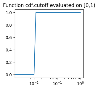
def cutoff(eigvals : np.ndarray, epsilon : float)

This function does the operation \(x\mapsto 1_{x\ge \varepsilon^2)}\). As before, the idea is that when applied to \(|\widehat{f}(\chi)|^2\) it is 1 only when \(|\widehat{f}(\chi)|\ge \varepsilon\).

plot_on_uniform_grid(cdf.cutoff, 0.1, 'cdf.cutoff')

# In hofa.cdf
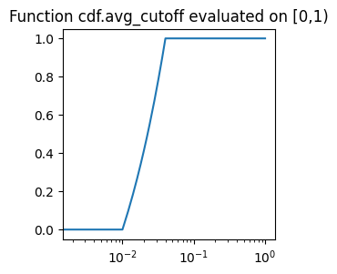
def avg_cutoff(eigvals : np.ndarray, epsilon : float)

This function is an averaged version of the previous one over the interval \([\rho,2\rho]\). Hence, it equals \(\mathbb{E}_{\varepsilon\in[\rho,2\rho]}1_{\sqrt{x}\ge \varepsilon}\). Equivalently, it is easy to deduce that it equals \(\min\big(\tfrac{\sqrt{\max(\rho^2,x)}}{\rho}-1,1\big)\).

plot_on_uniform_grid(cdf.avg_cutoff, 0.1, 'cdf.avg_cutoff')

# In hofa.cdf
def top_eig(eigvals : np.ndarray, n : int)

This function does not follow the pattern of the previous ones, as it does not assign a particular weight to the different eigenspaces but rather it masks for the top n eigenvalues. Note that an StandardLayerRegularizer class that uses it must also choose mode='literal' and provide such number.

# In hofa.cdf
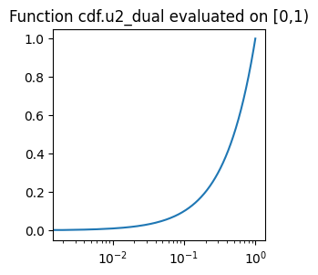
def u2_dual(eigvals : np.ndarray, unused : float)

Last but not least we have a function that corresponds to the \(U^2\) dual operator. It turns out that this is probably the simplest of all, \(x\mapsto x\) (the parameter unused is ignored). (Recall that we are putting a logaritmic scale in the \(x\) axis, that is why we do not see an straight line.)

plot_on_uniform_grid(cdf.u2_dual, 0.1, 'cdf.u2_dual')

The param and mode parameters

As we just said, there is a parameter \(\tau\) that each StandardLayerRegularizer object will use to pass to the alpha_method to compute the weights of the different eigenspaces. Suppose that a particular StandardLayerRegularizer object is called during setup with depth=\(k\) and layer=\(l\). Let param=\(C\), let \(f\) be the original function to regularize and let \(\Delta_{t_1}\cdots\Delta_{t_{k-l-1}}f\) be the particular function the StandardLayerRegularizer object has to regularize of order \(U^{l+1}\). The parameter \(\tau\) will then be computed as follows.

• If mode='literal', then \(\tau = C\),

• If mode='dynamic-original' then \(\tau = C\sigma^{2^{k-l-1}}\sqrt{\tfrac{\log |Z|}{|Z|}}\) where \(\sigma^2 = \text{Var}(f) = \mathbb{E}_{x\in Z} |f-\mathbb{E}_{x\in Z}f|^2\).

• If mode='dynamic-strict' then \(\tau = C\tilde{\sigma}\sqrt{\tfrac{\log |Z|}{|Z|}}\) where \(\tilde{\sigma}^2 = \text{Var}(\Delta_{t_1}\cdots\Delta_{t_{k-l-1}}f)\).

The heuristic explanation behind these options will be detailed in a forthcoming paper.

The lin_alg_method and the num_eigen parameters

These are used to allow the user to choose between two different methods for obtaining the eigenvalues and eigenvectors of a matrix. Recall that if layer=0 during setup these values will be ignored and instead the Fast Fourier Transform will be used. The possibilities are as follows.

• If lin_alg_method='full' then this regularizer will use numpy.linalg.eigh as the method for obtaining the eigenvalue decomposition. In this case, the parameter num_eigen is ignored.

• If lin_alg_method='sparse' and num_eigen is an integer, then this regularizer will use the method scipy.sparse.linalg.eigsh with the number of eigenvalues being precisely the number passed in num_eigen.

• If lin_alg_method='sparse' and num_eigen='dynamic', then this regularizer will use the method scipy.sparse.linalg.eigsh with the number of eigenvalues computed dynamically by the formula \(\lfloor \tfrac{|Z|}{C^2\log|Z|}\rfloor\) where the constant param=\(C\) as in the previous section.

Putting everything together: Chirps

Having described the main components of the package and how they interact, we now illustrate their use on a concrete example with chirps. This section demonstrates how the regularize function performs in a larger, more complicated example. We will follow the same structure as in our toy example at the beginning but with some changes.

Problem statement

We want to transmit a convex combination of a periodic linear chirp of period \(n=1001\) and a non-periodic linear chirp defined for \(\{0,\ldots,n-1\}\).

\[f_s(x)=\tfrac{1}{2}\sin(200\pi x^2/n)+\tfrac{1}{2}\sin(5x^2/n)\]

defined for any integer \(x\in\{0,\ldots,n-1\}\). Similarly as above, imagine that our communication channel introduces noise, and what is received is a convex combination \(f=tf_r+(1-t)f_s\) where \(f_r(x)\) follows a uniform distribution \(\text{Unif}([-1,1))\) independently for every integer \(x\) and the amount of noise is \(t\), a parameter that we are going to vary in \([0,1)\).

Objective

Under these assumptions, we aim to compute an estimate of \(f_s\).

This time, instead of using the default values of regularize, let us use a different alpha_method.

import moviepy as mpy
import os

N = 1001
output_video = '_output/tutorial_denoising.mp4'

def f_s(x : np.ndarray):
    return 0.5*np.sin(2*100*np.pi*x**2/N)+0.5*np.sin((5*x**2)/N)

# For the quadratic regularization we use now the average cutoff, and for computing the 
# eigendecomposition, we only use 6 dominant eigenvectors.
# We fix the random number generator for reproducibility.
list_reg = [
    rgz.StandardLayerRegularizer(alpha_method = cdf.avg_cutoff, rng = 28),
    rgz.StandardLayerRegularizer(alpha_method = cdf.avg_cutoff, rng = 28, num_eigen= 6)
]

Strategy

Let us run the regualrize() function on the noisy version of \(f_s\) for values of \(t\) in \([0,1)\). The resulting function will be our candidate for recovery of \(f_s\). Let us plot the function to approximate, the noisy version, and the regularized result in a video. You can find the video on the folder _output.

x_values = np.arange(N)
rng = np.random.default_rng(123)
r_values = rng.uniform(-1, 1, size=len(x_values))
frames = 100

# Function to generate a frame
def generate_frame(t):

    print(f"t: {t:.2f}",end='\r')
    
    # Compute f(x) for the selected window
    y_values = (1 - t) * f_s(x_values)
    
    # Compute the modified function f_mod(x) = (1-t)*f(x) + t*r(x) using the same r_values
    y_values_mod = y_values + t * r_values

    # Regularize with respect to quadratic Fourier analysis
    y_values_quad_reg = rgz.regularize(y_values_mod,list_reg).regularization
    
    # Create the plot
    fig, ax = plt.subplots(figsize=(12, 5))
    
    # Plot original function in light green with thin, semi-transparent lines and dots
    ax.plot(x_values, np.real(y_values), linestyle='-', color='lightgreen', marker='o', markersize=6, linewidth=1, alpha=0.6, label=fr'$(1-t)*f_s(x)$')
    
    # Plot modified function in red with thin, semi-transparent lines and dots
    ax.plot(x_values, np.real(y_values_mod), linestyle='-', color='red', marker='o', markersize=6, linewidth=1, alpha=0.6, label=r'$(1-t)f_s(x) + tf_r(x)$')

    # Plot recovered function with fourier analysis in yellow with thin, semi-transparent lines and dots
    ax.plot(x_values, np.real(y_values_quad_reg), linestyle='-', color='yellow', marker='o', markersize=3, linewidth=1, alpha=0.6, label=r'quadratic regularization')
    
    # Customize the plot
    ax.set_xlabel("x")
    l1_original = np.mean(np.abs(y_values))
    ax.set_title(f"t: {t:.2f}, \
    L1 original {l1_original:.5f},\
    L1 error quadratic reg. {np.mean(np.abs(y_values_quad_reg-y_values)):.5f}")
    ax.grid(True, linestyle="--", alpha=0.6)
    
    # Fix y-axis range and ticks from -1 to 1
    ax.set_ylim(-1, 1)
    ax.set_yticks(np.linspace(-1, 1, 5))  # Keeps y-axis ticks fixed at [-1, -0.5, 0, 0.5, 1]
    
    # Legend below the plot
    fig.subplots_adjust(bottom=0.25)  # Adjust layout to fit legend below
    ax.legend(loc='upper center', bbox_to_anchor=(0.5, -0.15), ncol=2, frameon=False)
    
    # Save frame as image
    filename = f"_output/frame_{t:.2f}.png"
    plt.savefig(filename)
    plt.close()
    return filename

# Generate frames
frame_files = [generate_frame(t / (frames - 1)) for t in range(frames)]

# Create movie
clip = mpy.ImageSequenceClip(frame_files, fps=10)
clip.write_videofile(output_video, codec='libx264')

# Remove individual frame images
for frame in frame_files:
    os.remove(frame)

print(f"Movie saved at {output_video}, individual frames deleted.")

MoviePy - Building video _output/tutorial_denoising.mp4.
MoviePy - Writing video _output/tutorial_denoising.mp4

MoviePy - Done !
MoviePy - video ready _output/tutorial_denoising.mp4
Movie saved at _output/tutorial_denoising.mp4, individual frames deleted.

Putting everything together: Coding theory

The previous example focused on the theory of chirps. In this section, we consider a different application that highlights the same algorithmic framework from a coding-theoretic perspective.

While the underlying workflow and API remain unchanged, this example emphasizes structural aspects that may be of particular interest to readers with a background in coding theory or discrete signal models. The goal is to illustrate how the general design presented above naturally accommodates this setting, without introducing additional mathematical machinery beyond what is strictly necessary.

Problem statement

We want to transmit a function \(\{0,1\}^{7}\to \{-1,1\}\) that can be expressed as a quadratic polynomial \(\mathbb{F}_2^{7}\to \mathbb{C}\)

\[f_s(x)= \exp( \pi i \sum_{i=0}^{5} x_ix_{i+1}).\]

Note that this functions equals \(1\) when \(\sum_{i=0}^{5} x_ix_{i+1}\) is even and \(-1\) when \(\sum_{i=0}^{5} x_ix_{i+1}\) is odd. Similar functions appear for example in the Reed-Muller codes.

Now imagine that we want to transmit the values of this function, but again out communication channel is noisy, and for a proportion \(t\in[0,1)\) of the values, it swaps \(1\) and \(-1\) with probability \(1/2\). Let us denote this noisy version of \(f_s\) by \(f\).

Objective

Under these assumptions, for different values of \(t\), we aim to compute an estimate of \(f_s\).

import moviepy as mpy
import os
import itertools

output_video2 = '_output/tutorial_denoising2.mp4'

n = 7
f_s = np.empty([2]*n).astype(complex)

def quadratic_poly(x : np.ndarray):
    return np.exp(np.pi*1j*np.sum(x[:-1]*x[1:]))

for idx in itertools.product([0, 1], repeat=n):
    f_s[idx] = np.real(quadratic_poly(np.array(idx)))

Now we create the function \(f\) for every \(t\) between \(0\) and \(1\) and we regularize it using our algorithm.

Strategy

While our original signal takes either \(1\) or \(-1\), this is no longer the case for the case of our regularized version. Thus, we may simply take the real part of our regularization and take 1 if the number is positive and -1 if it is negative. This is how we reconstruct our signal.

import random
import math

list_indices = list(itertools.product([0, 1], repeat=n))
M = len(list_indices)
rng = np.random.default_rng(4)
rng.shuffle(list_indices)
swapping_parameters = rng.integers(low = 0, high = 2, size = M)*2-1

frames = 100
x_values = range(M)

# Function to generate a frame
def generate_frame(t):

    print(f"t: {t:.2f}",end='\r')

    # We compute the noisy version of f_s
    elements_to_alter = math.floor(M*t)
    multipliers = np.ones_like(f_s)
    for i in range(elements_to_alter):
        multipliers[list_indices[i]] *= swapping_parameters[i]
    f = f_s*multipliers

    # Regularize with respect to quadratic Fourier analysis
    # Similarly as before, we fix the Random Number Generator for reproducibility
    y_values_quad_reg = np.sign(np.real(rgz.regularize(f,2, rng = 28).regularization))
    
    # Create the plot
    fig, ax = plt.subplots(figsize=(12, 5))
    
    # Plot original function in light green with thin, semi-transparent lines and dots
    ax.plot(x_values, np.real(f_s.flatten()), linestyle=None, color='lightgreen', marker='o', markersize=6, linewidth=1, alpha=0.6, label=fr'$(1-t)*f_s(x)$')
    
    # Plot modified function in red with thin, semi-transparent lines and dots
    ax.plot(x_values, np.real(f.flatten()), linestyle=None, color='red', marker='o', markersize=6, linewidth=1, alpha=0.6, label=r'$(1-t)f_s(x) + tf_r(x)$')

    # Plot recovered function with fourier analysis in yellow with thin, semi-transparent lines and dots
    ax.plot(x_values, np.real(y_values_quad_reg.flatten()), linestyle=None, color='yellow', marker='o', markersize=3, linewidth=1, alpha=0.6, label=r'quadratic regularization')
    
    # Customize the plot
    ax.set_xlabel("x")
    l1_original = np.mean(np.abs(f_s))
    ax.set_title(f"Perfectage of elements randomly swapped with probability 1/2: {elements_to_alter/M*100:.2f}%, \
    Percentage of failed reconstruction: {100*np.sum(y_values_quad_reg!=f_s)/M:.2f}%")
    ax.grid(True, linestyle="--", alpha=0.6)
    
    # Fix y-axis range and ticks from -1 to 1
    ax.set_ylim(-1.1, 1.1)
    ax.set_yticks(np.linspace(-1, 1, 5))  # Keeps y-axis ticks fixed at [-1, -0.5, 0, 0.5, 1]
    
    # Legend below the plot
    fig.subplots_adjust(bottom=0.25)  # Adjust layout to fit legend below
    ax.legend(loc='upper center', bbox_to_anchor=(0.5, -0.15), ncol=2, frameon=False)
    
    # Save frame as image
    filename = f"_output/frame_{t:.2f}.png"
    plt.savefig(filename)
    plt.close()
    return filename

# Generate frames
frame_files = [generate_frame(t / (frames - 1)) for t in range(frames)]

# Create movie
clip = mpy.ImageSequenceClip(frame_files, fps=10)
clip.write_videofile(output_video2, codec='libx264')

# Remove individual frame images
for frame in frame_files:
    os.remove(frame)

print(f"Movie saved at {output_video2}, individual frames deleted.")

MoviePy - Building video _output/tutorial_denoising2.mp4.
MoviePy - Writing video _output/tutorial_denoising2.mp4

MoviePy - Done !
MoviePy - video ready _output/tutorial_denoising2.mp4
Movie saved at _output/tutorial_denoising2.mp4, individual frames deleted.

Check the video we have just created, where up to a \(t=50\)% of randomly swapped parameters (that means that on average we have changed \(25\)% of the values) we get a perfect reconstruction.

Optional: deeper insights and extensions

Recall from Theoretical Foundations and Extensions that we mentioned some family of functions called nilsequences that in a sense work similarly as periodic quadratic polynomials but cannot be represented as those. The hofa package can also deal with this kind of functions.

A nilsequence

A 2-step nilsequence is a function which shares many properties with periodic quadratic polynomials (such as chirps or in general quadratic exponentials), but which cannot be decomposed or even approximated efficiently by functions of the form \(e^{2\pi i (ax^2+bx+c)/n}\) for integers \(a,b,c\). Nevertheless, a 2-step nilsequence has the property that it also has a non-trivial \(U^3\) norm. See Theoretical Foundations and Extensions for a lengthier presentation of these functions. To define them, we need to consider the Heisenberg group

\[\begin{split}G:=\left(\begin{matrix} 1 & \mathbb{R} & \mathbb{R}\\[0.1em]0 & 1 & \mathbb{R}\\[0.1em] 0 & 0 & 1 \end{matrix}\right) \text{ and the discrete Heisenberg group } \Gamma:=\left(\begin{matrix} 1 & \mathbb{Z} & \mathbb{Z}\\[0.1em]0 & 1 & \mathbb{Z}\\[0.1em] 0 & 0 & 1 \end{matrix}\right)\end{split}\]

The Heisenberg manifold is then \(G/\Gamma\). To define a nilsequence here, we let \(r\) be an integer and we let

\[\begin{split}M=\left(\begin{matrix} 1 & 2r/n & r/n^2\\[0.1em]0 & 1 & 1/n\\[0.1em] 0 & 0 & 1 \end{matrix}\right) \end{split}\]

Our nilsequence \(f_s:\mathbb{Z}\to \mathbb{C}\) is defined as follows. Let \(\{g\Gamma\}\) be thethe representative in \([0,1)\) of the top right corner of any element \(g\Gamma\) for \(g\in G\). Then \(f_s(x)=\exp(2\pi i \{M^x\Gamma\}) = \exp(2\pi i t x^2/n^2)\) for \(x=0,\ldots,n\). Note that, while this may look like a quadratic polynomial, it is not because we have a term \(n^2\) in the denominator. This seemingly unimportant detail is important, and ultimately tells us that a more complicated representation using the Heisenberg nilmanifold is necessary.

Problem statement

Similarly as with chirps, we will let \(f_s(x)=\exp(2\pi i \{M^x\Gamma\})\) for any integer \(x\) and we will modify it by taking a convex combination \(f=tf_r+(1-t)f_s\) where \(t\in[0,1)\) and \(f_r(x)\) follows a uniform distribution \(\text{Unif}([-1,1))\) independently for every integer \(x\).

Objective

Recover \(f_s\) from the noisy version \(f\).

import moviepy as mpy
import os

N = 1001
output_video = '_output/tutorial_denoising3.mp4'
t = 100

def f_s(x : np.ndarray):
    return np.exp(2*t*np.pi*1j*x**2/N**2)

x_values = np.arange(N)
rng = np.random.default_rng(123)
r_values = rng.uniform(-1, 1, size=len(x_values))
frames = 100

# Function to generate a frame
def generate_frame(t):

    print(f"t: {t:.2f}",end='\r')
    
    # Compute f(x) for the selected window
    y_values = (1 - t) * f_s(x_values)
    
    # Compute the modified function f_mod(x) = (1-t)*f(x) + t*r(x) using the same r_values
    y_values_mod = y_values + t * r_values

    # Regularize with respect to quadratic Fourier analysis
    y_values_quad_reg = rgz.regularize(y_values_mod,2).regularization
    
    # Create the plot
    fig, ax = plt.subplots(figsize=(12, 5))
    
    # Plot original function in light green with thin, semi-transparent lines and dots
    ax.plot(x_values, np.real(y_values), linestyle='-', color='lightgreen', marker='o', markersize=6, linewidth=1, alpha=0.6, label=fr'$(1-t)*f_s(x)$')
    
    # Plot modified function in red with thin, semi-transparent lines and dots
    ax.plot(x_values, np.real(y_values_mod), linestyle='-', color='red', marker='o', markersize=6, linewidth=1, alpha=0.6, label=r'$(1-t)f_s(x) + tf_r(x)$')

    # Plot recovered function with fourier analysis in yellow with thin, semi-transparent lines and dots
    ax.plot(x_values, np.real(y_values_quad_reg), linestyle='-', color='yellow', marker='o', markersize=3, linewidth=1, alpha=0.6, label=r'quadratic regularization')
    
    # Customize the plot
    ax.set_xlabel("x")
    l1_original = np.mean(np.abs(y_values))
    ax.set_title(f"t: {t:.2f}, \
    L1 original {l1_original:.5f},\
    L1 error quadratic reg. {np.mean(np.abs(y_values_quad_reg-y_values)):.5f}")
    ax.grid(True, linestyle="--", alpha=0.6)
    
    # Fix y-axis range and ticks from -1 to 1
    ax.set_ylim(-1, 1)
    ax.set_yticks(np.linspace(-1, 1, 5))  # Keeps y-axis ticks fixed at [-1, -0.5, 0, 0.5, 1]
    
    # Legend below the plot
    fig.subplots_adjust(bottom=0.25)  # Adjust layout to fit legend below
    ax.legend(loc='upper center', bbox_to_anchor=(0.5, -0.15), ncol=2, frameon=False)
    
    # Save frame as image
    filename = f"_output/frame_{t:.2f}.png"
    plt.savefig(filename)
    plt.close()
    return filename

# Generate frames
frame_files = [generate_frame(t / (frames - 1)) for t in range(frames)]

# Create movie
clip = mpy.ImageSequenceClip(frame_files, fps=10)
clip.write_videofile(output_video, codec='libx264')

# Remove individual frame images
for frame in frame_files:
    os.remove(frame)

print(f"Movie saved at {output_video}, individual frames deleted.")

MoviePy - Building video _output/tutorial_denoising3.mp4.
MoviePy - Writing video _output/tutorial_denoising3.mp4

MoviePy - Done !
MoviePy - video ready _output/tutorial_denoising3.mp4
Movie saved at _output/tutorial_denoising3.mp4, individual frames deleted.