What HoFa can do#
This tutorial will acquaint you with the main functionalities of the HoFa package, which are the following:
Detect higher-order structure in signals.
Denoise signals with respect to higher-order structure.
Decompose signals into dominant higher-order components.
NOTE: You will need the
HoFapackage installed before running this notebook, see the Installation guide. For a quick installation in a virtual environment (say, for example,hofavenv), run the following command:
(hofavenv) $ pip install hofa
Detect higher-order structure: the norm module#
The critical tools that we need for this section are the Gowers norms, also known as Gowers \(U^k\)-norms or \(U^k\)-norms for short. These norms tell us whether there is some hidden quadratic (or higher-order) structure in a signal.
As an example, let us consider three different signals \(f_1,f_2,f_3\) defined on \(\{0,1,\ldots,n-1\}\):
import hofa.norm
import numpy as np

n = 501

# For reproducibility, we fix a Random Number Generator
rng = np.random.default_rng(123)

x = np.arange(n)

f_1 = rng.uniform(-1, 1, size=n)
f_2 = np.sin(2*np.pi*x/n)
f_3 = np.sin(2*np.pi*x**2/n)
Let us now plot the signals:
import matplotlib.pyplot as plt

# Create a figure with 3 subplots side by side
fig, (ax1, ax2, ax3) = plt.subplots(1, 3, figsize=(15, 4))

# Plot each function in its own subplot
ax1.plot(x, f_1, label='Random uniform noise', color='blue')
ax1.set_title(r'$f_1$')
ax1.grid(True)
ax1.legend(loc='upper center', bbox_to_anchor=(0.5, -0.15), ncol=2, frameon=False)  # Display the legend for the first subplot

ax2.plot(x, f_2, label=r'$\sin(2\pi x/n)$', color='red')
ax2.set_title(r'$f_2$')
ax2.grid(True)
ax2.legend(loc='upper center', bbox_to_anchor=(0.5, -0.15), ncol=2, frameon=False)  # Display the legend for the first subplot

ax3.plot(x, f_3, label=r'$\sin(2\pi x^2/n)$', color='green')
ax3.set_title(r'$f_3$')
ax3.grid(True)
ax3.legend(loc='upper center', bbox_to_anchor=(0.5, -0.15), ncol=2, frameon=False)  # Display the legend for the first subplot

# Adjust layout to prevent overlap
plt.tight_layout()
plt.show()
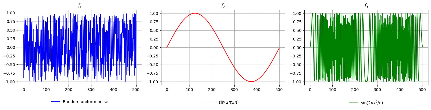
Clearly the three plots are different, but the first and third signals seem to have something in common: they both look like noise. Moreover, if we analyze such functions using the Fourier transform, we find that those two signals share the following interesting feature: all of their Fourier amplitudes are small, as we can see in the following plot.
NOTE: We use the convention that, given a function \(f:\{0,\ldots,n-1\}\to\mathbb{C}\) and a Fourier character \(\chi\), the Fourier coefficient of \(f\) at frequency \(\chi\) is given by
# Compute Fourier transforms
fft_1 = np.fft.fft(f_1, norm="forward")
fft_2 = np.fft.fft(f_2, norm="forward")
fft_3 = np.fft.fft(f_3, norm="forward")

# Create a figure with 3 subplots side by side
fig, (ax1, ax2, ax3) = plt.subplots(1, 3, figsize=(15, 5))

# Plot absolute values of Fourier transforms
ax1.plot(x, np.abs(fft_1), label=r'$|\widehat{f_1}|$', color='blue')
ax1.set_xlabel('Frequency')
ax1.set_ylabel('Magnitude')
ax1.grid(True)
ax1.legend(loc='upper center', bbox_to_anchor=(0.5, -0.2))
ax1.set_ylim(-1, 1)

ax2.plot(x, np.abs(fft_2), label=r'$|\widehat{f_2}|$', color='red')
ax2.set_xlabel('Frequency')
ax2.grid(True)
ax2.legend(loc='upper center', bbox_to_anchor=(0.5, -0.2))
ax2.set_ylim(-1, 1)

ax3.plot(x, np.abs(fft_3), label=r'$|\widehat{f_3}|$', color='green')
ax3.set_xlabel('Frequency')
ax3.grid(True)
ax3.legend(loc='upper center', bbox_to_anchor=(0.5, -0.2))
ax3.set_ylim(-1, 1)

# Adjust layout to prevent overlap
plt.tight_layout(rect=[0, 0, 1, 0.95])
plt.show()
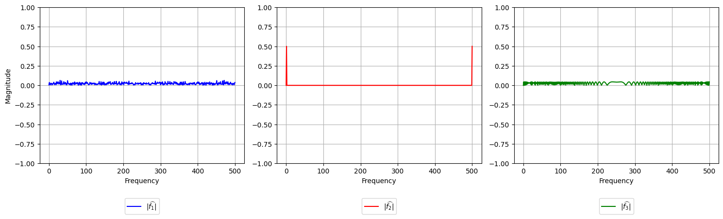
Despite their similarity from the classical Fourier analytic viewpoint, the first and third signals are clearly not the same, the first signal is completely random noise whereas the third has quadratic behavior. Distinguishing this in a systematic way is precisely what the Gowers norms will enable. The Gowers norms are a family of norms defined on the space of functions \(f:\{0,\ldots,N-1\}\to\mathbb{C}\) (or more general domains) that capture the following features:
The Gowers \(U^1\)-seminorm captures the average behavior: how large is the average of a function; in particular, whether the function has a significant part that can be expressed as a constant.
The Gowers \(U^2\)-norm captures linear behavior: how sensitive is the function to (classical) Fourier-analytic methods; in particular, whether a significant part of it can be sparsely decomposed with functions of the form \(\exp(2\pi i \xi x)\).
The Gowers \(U^3\)-norm captures quadratic behavior: in particular, whether a function has a significant part that can be sparsely decomposed with quadratic harmonics such as \(\exp(2\pi i (\xi x^2+\xi'x))\).
The Gowers \(U^4\)-norm…
NOTE: The Gowers \(U^1\)-seminorm can be seen to fit into the scheme of the higher-order norms, in that it detects whether a function has a significant part that can be expressed as a multiple of \(\exp(2\pi i \xi x^0)\), i.e. of a constant function. It is a common abuse of notation to talk about the Gowers \(U^k\)-norms collectively even though the case \(k=1\) is only a seminorm (it is also common to refer to the \(U^1\)-seminorm simply as the \(U^1\)-norm).
The formal definition of the Gowers norms is provided in this documentation in the conceptual and mathematical background of higher-order Fourier analysis.
Observation: The Gowers \(U^k\)-norms (\(k\ge 1\)) form an increasing sequence of norms. That is, for a functon \(f\), if we let \(\|f\|_{U^k}\) denote its \(U^k\)-norm, then \(\|f\|_{U^1}\le \|f\|_{U^2}\le \|f\|_{U^3}\le\cdots\). This aligns with the picture described before; e.g. having some non-trivial linear (classical Fourier) structure implies having quadratic structure, as functions of the form \(\exp(2\pi i (\xi x^2+\xi'x))\) already include the linear cases \(\exp(2\pi i \xi'x)\) (just by setting \(\xi=0\)).
The HoFa package can be used to compute the Gowers norms; let us compute them for the examples \(f_1,f_2,f_3\) above:
norm_axis = np.arange(1,4)

# Compute y-values for each array
y1 = [hofa.norm.u(f_1, i) for i in norm_axis]
y2 = [hofa.norm.u(f_2, i) for i in norm_axis]
y3 = [hofa.norm.u(f_3, i) for i in norm_axis]

# Plot
plt.plot(norm_axis, y1, marker='o', label=r'$f_1$')
plt.plot(norm_axis, y2, marker='o', label=r'$f_2$')
plt.plot(norm_axis, y3, marker='o', label=r'$f_3$')

# Labels and legend
plt.xlabel('order $k$ of the Gowers norm')
plt.ylabel(r'value of the Gowers norm of $f$')
plt.xticks(norm_axis)
plt.legend()
plt.grid(True)

plt.show()
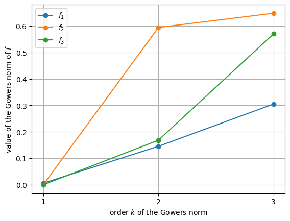
Note the significant differences between the \(U^2\)-norms and \(U^3\)-norms of these functions. In general, if a function has a \(U^k\)-norm that is non-trivially large (and thus markedly different from the \(U^k\)-norm of random \([-1,1]\)-valued noise), then this signals the presence of some kind of structure of order \(k-1\) in the function. Let us analyze the above example in this light:
As \(\|f_2\|_{U^2}\) is significantly larger than \(\|f_1\|_{U^2}\), this signals the presence of linear (classical Fourier) structure in \(f_2\).
As \(\|f_3\|_{U^2}\) is similar to \(\|f_1\|_{U^2}\), this signals that, relative to (classical) Fourier analysis, the signals are similar.
As \(\|f_3\|_{U^3}\) is significantly larger than \(\|f_1\|_{U^3}\), this signals the presence of quadratic structure in \(f_3\).
Denoise signals with respect to higher-order structure#
Usually, signals in real scenarios do not come in such neatly distinct ways as in the previous example. Instead, what we commonly encounter is a superposition of the structured signal with some added noise. Continuing with the examples \(f_1(x)\sim\text{Unif}(-1,1)\) and \(f_3(x)=\sin(2\pi x^2/n)\), imagine that we are trying to send the signal \(f_3\) but the channel which we use introduces a \(t=50\%\) noise (represented by the function \(f_1\)). Then, at the receptor we receive
t = 0.5

g = (1-t)*f_3+t*f_1
The HoFa package includes a Regularization method that helps to recover the quadratically structured component \((1-t)f_2\). Note that Fourier based methods are of little use for this, as the Fourier transforms of \(f_1\) and \(f_3\) are very small and the Fourier transform of the perturbed version \(g\) need not be similar to the Fourier transform of \(f_3\).
The method that enables the mentioned recovery is hofa.rgz.regularize:
import hofa.rgz

regularized_g = np.real(hofa.rgz.regularize(g,2).regularization)
Let us now plot the results:
# Create a figure with 3 subplots side by side
fig, (ax1, ax2, ax3) = plt.subplots(1, 3, figsize=(15, 4))

# Plot each function in its own subplot
ax1.plot(x, g, label=r'$(1-t)f_3+tf_1$', color='blue')
ax1.set_title(r'$g$')
ax1.grid(True)
ax1.legend(loc='upper center', bbox_to_anchor=(0.5, -0.15), ncol=2, frameon=False)  # Display the legend for the first subplot
ax1.set_ylim(-1, 1)

ax2.plot(x, (1-t)*f_3, label=r'$(1-t)\sin(2\pi x^2/n)$', color='red')
ax2.set_title(r'$(1-t)f_3$')
ax2.grid(True)
ax2.legend(loc='upper center', bbox_to_anchor=(0.5, -0.15), ncol=2, frameon=False)  # Display the legend for the first subplot
ax2.set_ylim(-1, 1)

ax3.plot(x, regularized_g, label=r'Recovered signal', color='green')
ax3.set_title(r'Output of `hofa.rgz.regularize`')
ax3.grid(True)
ax3.legend(loc='upper center', bbox_to_anchor=(0.5, -0.15), ncol=2, frameon=False)  # Display the legend for the first subplot
ax3.set_ylim(-1, 1)

# Adjust layout to prevent overlap
plt.tight_layout()
plt.show()

print(f'L^1 difference between (1-t)f_3 and the output: {np.abs(np.mean(regularized_g-(1-t)*f_3))}')
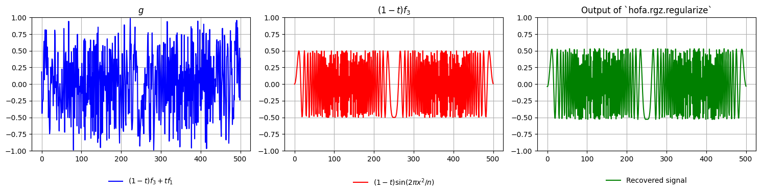
L^1 difference between (1-t)f_3 and the output: 0.0016458352513586331
Decompose signals into their higher-order components#
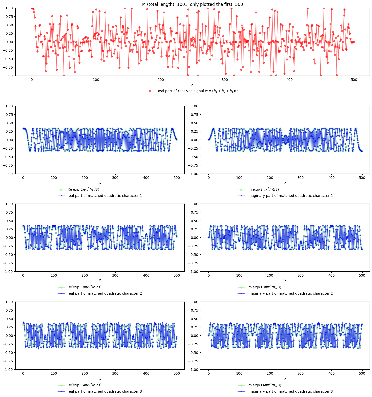
Finally, HoFa enables us to decompose functions into their higher-order components. Imagine that we are now sending three chirps \(h_1,h_2,h_3:\{0,\ldots,M-1\}\to \mathbb{C}\), for \(M=1001\), defined as follows:
but our receptor has received at once the three chirps superposed, i.e. we receive \(w=(h_1+h_2+h_3)/3\).
M = 1001
x = np.arange(M)

h_1 = np.exp(2*np.pi*1j*x**2/M)
h_2 = np.exp(10*np.pi*1j*x**2/M)
h_3 = np.exp(14*np.pi*1j*x**2/M)

w = (h_1+h_2+h_3)/3
The HoFa package includes a Spectral higher-order Fourier transform implemented in hofa.char.spechoft that can identify and separate the different quadratic components of this example.
import hofa.char

# As usual, we fix a Random Number Generator for reproducibility
rnd_sep_result = hofa.char.spechoft(w, order = 2, rng=28)

eichars = rnd_sep_result.higher_order_char
Let us plot the result of this function against the known underlying functions \(h_1,h_2,h_3\). Note that hofa.char.spechoft does not return the different components in a particular order. Thus, we have to find the most appropriate order for better visualization.
import itertools

# For convenience, we only plot the first 500 elements of each function
number_of_first_elems_to_plot = 500

v_1 = eichars[:, -1]
coeff_proj_1 = np.mean(w * v_1.conjugate())

v_2 = eichars[:, -2]
coeff_proj_2 = np.mean(w * v_2.conjugate())

v_3 = eichars[:, -3]
coeff_proj_3 = np.mean(w * v_3.conjugate())

# Restrict to plotting window
x_plot = x[:number_of_first_elems_to_plot]

# Target ("green") complex curves
target_1_complex = h_1 / 3
target_2_complex = h_2 / 3
target_3_complex = h_3 / 3

targets_complex = [target_1_complex, target_2_complex, target_3_complex]

# Recovered ("blue") complex curves
blue_1_complex = coeff_proj_1 * v_1#[:number_of_first_elems_to_plot]
blue_2_complex = coeff_proj_2 * v_2#[:number_of_first_elems_to_plot]
blue_3_complex = coeff_proj_3 * v_3#[:number_of_first_elems_to_plot]

blues_complex = [blue_1_complex, blue_2_complex, blue_3_complex]

# --- L^2 (squared) error comparison over all 3! possible assignments ---
# Match using the full complex-valued curves

best_perm = None
best_err = np.inf

for perm in itertools.permutations(range(3)):
    total_err = sum(
        np.sum(np.abs(blues_complex[perm[i]] - targets_complex[i])**2)
        for i in range(3)
    )
    if total_err < best_err:
        best_err = total_err
        best_perm = perm

# Reorder blues according to best assignment
matched_blues_complex = [blues_complex[best_perm[i]] for i in range(3)]

# Labels
target_labels_real = [
    r'$\mathrm{Re}\!\left(\exp(2\pi i x^2/n)/3\right)$',
    r'$\mathrm{Re}\!\left(\exp(10\pi ix^2/n)/3\right)$',
    r'$\mathrm{Re}\!\left(\exp(14\pi ix^2/n)/3\right)$',
]

target_labels_imag = [
    r'$\mathrm{Im}\!\left(\exp(2\pi i x^2/n)/3\right)$',
    r'$\mathrm{Im}\!\left(\exp(10\pi ix^2/n)/3\right)$',
    r'$\mathrm{Im}\!\left(\exp(14\pi ix^2/n)/3\right)$',
]

blue_labels_real = [
    r"real part of matched quadratic character 1",
    r"real part of matched quadratic character 2",
    r"real part of matched quadratic character 3",
]

blue_labels_imag = [
    r"imaginary part of matched quadratic character 1",
    r"imaginary part of matched quadratic character 2",
    r"imaginary part of matched quadratic character 3",
]
Finally, we can plot the results once we have the best matching between the components found by hofa.char.spechoft and the original functions \(h_1,h_2,h_3\).
# --- Plotting ---

# 4 rows x 2 columns:
# top row spans both columns,
# then 3 rows of 2 plots each
fig = plt.figure(figsize=(15, 16))
gs = fig.add_gridspec(4, 2, height_ratios=[1, 1, 1, 1], width_ratios=[1, 1])

# Top plot
ax_top = fig.add_subplot(gs[0, :])
ax_top.plot(
    x_plot,
    np.real(w[:number_of_first_elems_to_plot]),
    linestyle="-",
    color="red",
    marker="o",
    markersize=5,
    linewidth=1,
    alpha=0.6,
    label=r"Real part of received signal $w=(h_1+h_2+h_3)/3$",
)
ax_top.set_xlabel("x")
ax_top.set_title(f"M (total length): {M}, only plotted the first: {number_of_first_elems_to_plot}")
ax_top.set_ylim(-1, 1)
ax_top.legend(loc="upper center", bbox_to_anchor=(0.5, -0.15), ncol=2, frameon=False)

# Bottom 3x2 comparison plots
for i in range(3):
    target = targets_complex[i]
    blue = matched_blues_complex[i]

    # Left: real parts
    ax_real = fig.add_subplot(gs[i + 1, 0])
    ax_real.plot(
        x_plot,
        np.real(target[:number_of_first_elems_to_plot]),
        linestyle="-",
        color="lightgreen",
        marker="o",
        markersize=5,
        linewidth=1,
        alpha=0.6,
        label=target_labels_real[i],
    )
    ax_real.plot(
        x_plot,
        np.real(blue[:number_of_first_elems_to_plot]),
        linestyle="-",
        color="blue",
        marker="o",
        markersize=3,
        linewidth=1,
        alpha=0.6,
        label=blue_labels_real[i],
    )
    ax_real.set_xlabel("x")
    ax_real.set_ylim(-1, 1)
    ax_real.legend(loc="upper center", bbox_to_anchor=(0.5, -0.15), ncol=1, frameon=False)

    # Right: imaginary parts
    ax_imag = fig.add_subplot(gs[i + 1, 1])
    ax_imag.plot(
        x_plot,
        np.imag(target[:number_of_first_elems_to_plot]),
        linestyle="-",
        color="lightgreen",
        marker="o",
        markersize=5,
        linewidth=1,
        alpha=0.6,
        label=target_labels_imag[i],
    )
    ax_imag.plot(
        x_plot,
        np.imag(blue[:number_of_first_elems_to_plot]),
        linestyle="-",
        color="blue",
        marker="o",
        markersize=3,
        linewidth=1,
        alpha=0.6,
        label=blue_labels_imag[i],
    )
    ax_imag.set_xlabel("x")
    ax_imag.set_ylim(-1, 1)
    ax_imag.legend(loc="upper center", bbox_to_anchor=(0.5, -0.15), ncol=1, frameon=False)

fig.tight_layout()
plt.show()